Before we get started, I want to introduce my favorite set-returning functions which can help you to generate sample data:
|
1 2 3 4 5 6 7 8 9 10 11 12 13 14 |
test=# SELECT * FROM generate_series(1, 10) AS x; x ---- 1 2 3 4 5 6 7 8 9 10 (10 rows) |
All we do here is to generate a list from 1 to 10 and print it on the screen. Let us play around with window functions a bit now: There are two cases we need to keep in mind. If the OVER-clause is empty it means that the entire data set is used. If we use ORDER BY, it is only the data set up to the current row in the sorted list. The following listing contains an example:
|
1 2 3 4 5 6 7 8 9 10 11 12 13 14 15 16 17 |
test=# SELECT *, array_agg(x) OVER (), array_agg(x) OVER (ORDER BY x) FROM generate_series(1, 10) AS x; x | array_agg | array_agg ----+------------------------+------------------------ 1 | {1,2,3,4,5,6,7,8,9,10} | {1} 2 | {1,2,3,4,5,6,7,8,9,10} | {1,2} 3 | {1,2,3,4,5,6,7,8,9,10} | {1,2,3} 4 | {1,2,3,4,5,6,7,8,9,10} | {1,2,3,4} 5 | {1,2,3,4,5,6,7,8,9,10} | {1,2,3,4,5} 6 | {1,2,3,4,5,6,7,8,9,10} | {1,2,3,4,5,6} 7 | {1,2,3,4,5,6,7,8,9,10} | {1,2,3,4,5,6,7} 8 | {1,2,3,4,5,6,7,8,9,10} | {1,2,3,4,5,6,7,8} 9 | {1,2,3,4,5,6,7,8,9,10} | {1,2,3,4,5,6,7,8,9} 10 | {1,2,3,4,5,6,7,8,9,10} | {1,2,3,4,5,6,7,8,9,10} (10 rows) |
As you can see, the last column keeps accumulating more values.
Often it is necessary to limit the set of data (the window) used by the window function. ROWS BETWEEN … PRECEDING … AND … FOLLOWING allows you to do exactly that. The following example shows how this works:
|
1 2 3 4 5 6 7 8 9 10 11 12 13 14 |
test=# SELECT *, array_agg(x) OVER (ORDER BY x ROWS BETWEEN 1 PRECEDING AND 1 FOLLOWING) FROM generate_series(1, 10) AS x; x | array_agg ----+----------- 1 | {1,2} 2 | {1,2,3} 3 | {2,3,4} 4 | {3,4,5} 5 | {4,5,6} 6 | {5,6,7} 7 | {6,7,8} 8 | {7,8,9} 9 | {8,9,10} 10 | {9,10} (10 rows) |
What you see is that the data fed to array_agg is seriously restricted. But the restriction we are using here is a static one. The constants are hardwired. In some cases, you might need more flexibility.
More often than not, configuration has to be determined on the fly. The beauty is that in PostgreSQL you can use a subselect as part of the OVER-clause, which gives you a lot of flexibility.
Before we move on to a demo, we need to create a configuration table:
|
1 2 3 4 |
test=# CREATE TABLE t_config (key text, val int); CREATE TABLE test=# INSERT INTO t_config VALUES ('before', 1), ('after', 2); INSERT 0 2 |
To make it simple, I've simply created two entries. The following SELECT statement uses those configuration parameters to do its magic. Here is how it works:
|
1 2 3 4 5 6 7 8 9 10 11 12 13 14 15 16 17 18 19 20 21 22 23 |
test=# SELECT *, array_agg(x) OVER (ORDER BY x ROWS BETWEEN (SELECT val FROM t_config WHERE key = 'before') PRECEDING AND (SELECT val FROM t_config WHERE key = 'after') FOLLOWING) FROM generate_series(1, 10) AS x; x | array_agg ----+------------ 1 | {1,2,3} 2 | {1,2,3,4} 3 | {2,3,4,5} 4 | {3,4,5,6} 5 | {4,5,6,7} 6 | {5,6,7,8} 7 | {6,7,8,9} 8 | {7,8,9,10} 9 | {8,9,10} 10 | {9,10} (10 rows) |
As you can see, the query performs as expected and can be configured dynamically.
Another important note: PARTITION BY can take not only a column, but also an expression, to split the data set. Many people are not aware of this feature, which is actually quite useful. Here is an example:
|
1 2 3 4 5 6 7 8 9 10 11 12 13 14 |
test=# SELECT *, array_agg(x) OVER (PARTITION BY x % 2) FROM generate_series(1, 10) AS x; x | array_agg ----+-------------- 10 | {10,2,4,6,8} 2 | {10,2,4,6,8} 4 | {10,2,4,6,8} 6 | {10,2,4,6,8} 8 | {10,2,4,6,8} 9 | {9,7,3,1,5} 7 | {9,7,3,1,5} 3 | {9,7,3,1,5} 1 | {9,7,3,1,5} 5 | {9,7,3,1,5} (10 rows) |
In this case, we had no problem splitting the data into odd and even numbers. What I want to point out here is that PostgreSQL offers a lot of flexibility. We encourage you to test it out for yourself.
Window functions are super important if you need to relate the rows in a result set to each other. You order them, you partition them, and then you define a window from which you can compute additional result columns.
Sometimes, you want to find out more about a timeseries. One thing we have seen quite often recently is to count how often somebody was active for a certain amount of time. “Detecting continuous periods of activity” will show you how to calculate these things in PostgreSQL easily.
In order to receive regular updates on important changes in PostgreSQL, subscribe to our newsletter, or follow us on Twitter, Facebook, or LinkedIn.
The functionality of using table partitions to speed up queries and make tables more manageable as data amounts grow has been available in Postgres for a long time already. Nicer declarative support became available from v10 on - so in general it’s a known technique for developers. But what is not so uniformly clear is the way how low-level partition management is done. Postgres leaves it up to users, but no real standard tools or even concepts have emerged.
So it happened again that a customer approached me with a plan to use partitions for an action logging use case. The customer couldn't find a nice tool to his liking after a session of googling and was looking for some advice. Sure I know some tools. But my actual advice seemed quite unconventional and surprising for him: Why all the craziness with tools for this simple task? Why not throw together and use something simple yourself?
Of course tools in a broader sense are necessary and great, we wouldn’t be here today without our stone axes. Software developers thrive on the skillful use of editors, programming languages, etc. But the thing with tools is that you should really know when you actually need to use one! And when it comes to simple, isolated tasks I’d argue that it’s better to delay picking one up until you absolutely need one, and understand the “problem space” on a sufficiently good level.
Adopting some deeply integrated software tools also bring risks to the table - like the added additional complexity. When something then goes sour you're usually up for some serious sweating / swearing as you quickly need to gain a deep understanding of the tool’s internals (as it was mostly set up some X months or years ago and who remembers all this stuff). That's a tough thing to do when the production database is unable to process user queries and your manager is breathing down your neck.
Also, most tools or products in the PostgreSQL realm are in the end just GitHub repos with code, but without the associated business model and support services behind them. Which means you can forget about any guarantees / SLA-s whatsoever unless you’re covered by some Postgres support provider. Even then not all 3rd party tools / extensions fall under the SLA, typically.
But sure - if you evaluate the associated dangers, learn the basics, evaluate the project liveliness (a must for Open Source tools I think) you could look for some tools that more or less automatically take care of the tasks needed. For PostgreSQL partitioning tasks, by the way, I think the most common ones are pg_partman and the very similarly named pg_pathman.
Disclaimer - this approach can only be recommended if you’re familiar with the problem space and have some programming skills, or actually rather SQL skills when it comes to database partitioning. What I wanted to show with this blog post is that it’s not really hard to do. That's true at least for the simple task of table partitioning, and I personally prefer this way over some more complex tools, where by the time you’re done with the README and digested all the concepts and configuration options, you could have actually written and tested the whole code needed. So below find some sample code describing one approach for how to implement your own time-based (the most common partition scheme I believe) partition management - i.e. pre-creating new partitions for future time ranges and dropping old partitions.
From the business logic side let’s assume here that we have a schema for capturing millions of user interaction events per day (not uncommon for bigger shops), but luckily we need to store those events only for 6 months - a perfect use case for partitions!
|
1 2 3 4 5 6 7 8 9 |
CREATE TABLE event ( created_on timestamptz NOT NULL DEFAULT now(), user_id int8 NOT NULL, data jsonb NOT NULL ) PARTITION BY RANGE (created_on); CREATE INDEX ON event USING brin (created_on); CREATE EXTENSION IF NOT EXISTS btree_gin; CREATE INDEX ON event USING gin (user_id); |
That way we can get going and send to application to QA and have some time to figure out how we want to solve the future automation part. NB! Note that I’m creating a separate schema for the sub-partitions! This is actually a best practice, when it’s foreseeable that the amount of partitions is going to be more than a dozen or so (not the case for our demo schema though), so that they’re out of sight if we inspect our schema with some query tool and table access is still going to happen over the main table so partitions can be considered implementation details.
|
1 2 3 |
-- partitions for the current and next month CREATE SCHEMA subpartitions; CREATE TABLE event_y2020m05 PARTITION OF event FOR VALUES FROM ('2020-05-01') TO ('2020-06-01'); |
So now to the most important bits - creating new partitions and dropping old ones. The below query generates as SQL so that, when executed (for example by uncommenting the ‘gexec’ directive when using psql), it pre-creates a partition for the next month. When run as a weekly Cron, it should be enough.
|
1 2 3 4 5 6 7 8 9 10 11 12 13 14 15 16 17 18 19 20 21 22 23 24 25 |
WITH q_last_part AS ( select /* extract partition boundaries and take the last one */ *, ((regexp_match(part_expr, $$ TO ('(.*)')$$))[1])::timestamptz as last_part_end from ( select /* get all current subpartitions of the 'event' table */ format('%I.%I', n.nspname, c.relname) as part_name, pg_catalog.pg_get_expr(c.relpartbound, c.oid) as part_expr from pg_class p join pg_inherits i ON i.inhparent = p.oid join pg_class c on c.oid = i.inhrelid join pg_namespace n on n.oid = c.relnamespace where p.relname = 'event' and p.relkind = 'p' ) x order by last_part_end desc limit 1 ) SELECT format($$CREATE TABLE IF NOT EXISTS subpartitions.event_y%sm%s PARTITION OF event FOR VALUES FROM ('%s') TO ('%s')$$, extract(year from last_part_end), lpad((extract(month from last_part_end))::text, 2, '0'), last_part_end, last_part_end + '1month'::interval) AS sql_to_exec FROM q_last_part; -- gexec |
|
1 2 3 4 5 6 7 8 9 10 11 12 13 14 15 16 17 18 19 20 |
SELECT format('DROP TABLE IF EXISTS %s', subpartition_name) as sql_to_exec FROM ( SELECT format('%I.%I', n.nspname, c.relname) AS subpartition_name, ((regexp_match(pg_catalog.pg_get_expr(c.relpartbound, c.oid), $$ TO ('(.*)')$$))[1])::timestamptz AS part_end FROM pg_class p JOIN pg_inherits i ON i.inhparent = p.oid JOIN pg_class c ON c.oid = i.inhrelid JOIN pg_namespace n ON n.oid = c.relnamespace WHERE p.relname = 'event' AND p.relkind = 'p' AND n.nspname = 'subpartitions' ) x WHERE part_end < current_date - '6 months'::interval ORDER BY part_end; |
For real production use I’d recommend wrapping such things into nice, descriptively named stored procedures. Then, call them from good old Cron jobs or maybe also use the pg_cron extension if you have it installed already, or try out pg_timetable (our job scheduling software with advanced rules / chaining) or similar. Also don’t forget to set up some alerting and re-try mechanisms for production usage, as some hiccups will sooner or later appear - table locking issues on partition attaching / dropping, accidentally killed sessions etc.
And for multi-role access models I’d also recommend setting up reasonable DEFAULT PRIVILEGES for your schemas involved. That way all necessary application users will automatically gain correct access rights to new subpartition tables. This is not actually directly related to partitioning and is a good thing to set up for any schema.
For a lot of environments the simple task of running periodic jobs is actually not so simple - for example the environment might be very dynamic, with database and scheduling nodes jumping around the infrastructure and connectivity might become a problem, scheduling nodes might have different criticality classes and thus no access, etc. For such cases there are also some alternative partitioning tricks that can be applied. Mostly they look something like that:
If the volume of inserts is not too great it’s more or less OK to call the partition management code transparently in the background via triggers. The trigger will then look a bit into the future and pre-create the next sub-partitions on-the-fly, if not already existing - applying some dynamic SQL techniques usually.
For non-native (pre v10, inheritance based) partitioning you could also look into the actual row (see here for a code sample) and verify / create only the required partitions, but the newer declarative partition mechanism doesn’t allow “before” triggers, so you need to look into the future a bit.
Although from a performance point of view the previous method does not hurt as much as it might seem, as system catalog info is highly likely to be cached and mostly we don’t also need to create or drop any partitions, but under heavy volumes it could still start to hurt so a better idea might be to apply the whole partition management procedure only for a fraction of rows - most commonly by using the builtin random() function. Note that in this case a good trick is to apply the randomness filter (0.1% might be a good starting choice) at trigger definition level (the WHEN clause), not at trigger function level - this again saves some CPU cycles.
To formulate some kind of a “takeaway” for this post - we saw above that partition management can basically be implemented with only 2 SQL statements (without validation and retry mechanisms) - so why tie yourself to some 3rd party project X that basically doesn’t give you any guarantees, needs maybe installation of an extension and might make you wait before adding compatibility for some newly released PostgreSQL version?
We are so used to using all kinds of tools for everything and being always on the lookout for quick wins and those very rare “silver bullets” that we sometimes forget to stop and ask - do I really need a tool or an utility for the task at hand?
So my advice - if the task looks relatively simple, try to stop and rethink your needs. Is the new tool “investment” really worth it? What percentage of features of the tool are you actually interested in? And in a lot of cases when dealing with PostgreSQL you’ll see that things are not really that difficult to implement by yourself...and by doing so your system will gain one very important attribute - you stay in full control, know exactly what’s going on, and can easily make changes if needed.
Read on to find out more about partitioning in these posts:
In order to receive regular updates on important changes in PostgreSQL, subscribe to our newsletter, or follow us on Twitter, Facebook, or LinkedIn.
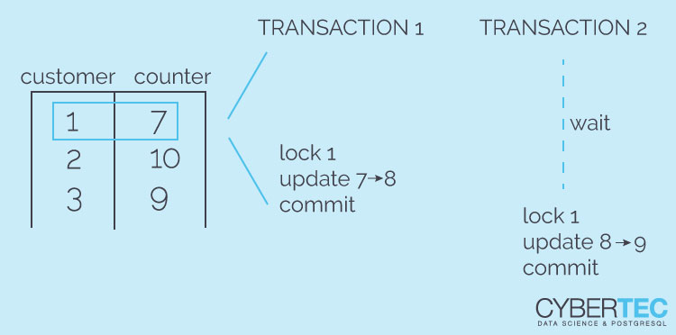
Concurrent counting in PostgreSQL: Recently we covered “count” quite extensively in this blog. We discussed optimizing count(*) and also talked about “max(id) - min(id)” which is of course a bad idea to count data in any relational database (not just in PostgreSQL). Today I want to focus your attention on a different kind of problem and its solution: Suppose you want to grant a user access to a certain piece of data only a limited number of times. How can you safely implement that?
One might argue that this is easy. Here is some pseudo code:
|
1 2 3 4 5 6 7 8 9 10 11 12 |
BEGIN; SELECT count(*) FROM log WHERE customer_id = 10 AND tdate = '2020-04-09' if count >= limit ROLLBACK else INSERT INTO log “do some work” COMMIT; |
Looks easy, doesn't it? Well, not really.
What happens if two people run this concurrently. Both sessions will receive the same result for count(*) and therefore one session will come to the wrong conclusion. Both transactions will proceed and do the work even if only one is allowed to do it. That is clearly a problem.
To solve the problem one could do ...
|
1 |
LOCK TABLE log IN ACCESS EXCLUSIVE MODE; |
... to eliminate concurrency all together. But, this is clearly a problem because it would block pg_dump or some analytics jobs or even VACUUM. Obviously not an attractive option. Alternatively we could try a SERIALIZABLE transaction but that might lead to many transactions failing due to concurrency issue.
One more problem is that count(*) might be really slow if there are already many entries. In short this approach has many problems:
But how can we do better?
To solve the problem we can introduce a “count table” but let us start right at the beginning. Let me create a table structure first:
|
1 2 3 4 5 6 7 8 9 10 11 12 13 14 15 16 17 18 19 20 21 |
CREATE EXTENSION btree_gist; CREATE TABLE t_customer ( id serial PRIMARY KEY, customer_email text NOT NULL UNIQUE, login_whatever_else text ); CREATE TABLE t_customer_limit ( id serial PRIMARY KEY, customer_id int REFERENCES t_customer (id) ON UPDATE CASCADE ON DELETE SET NULL, clicks_per_day int CHECK (clicks_per_day > 0) NOT NULL, trange tstzrange, EXCLUDE USING gist (trange WITH &&, customer_id WITH =) ); CREATE INDEX idx_limit ON t_customer_limit(customer_id); |
First of all I have installed an extension which is needed for one of the tables (more on that later).The customer table contains an id, some login email address and some other fields for whatever purpose. Note that this is mostly a prototype implementation.
Then comes an important table: t_customer_limit. It tells us how many clicks per day which customer can have. PostgreSQL supports “range types”. A period can be stored in a single column. Using range types has a couple of advantages. PostgreSQL will automatically check if the period is valid (end > start and so on). In addition to that the database provides a couple of operators to make handling really easy.
In the next step I have created a table to track all requests thrown at us. Creating such a table has the advantage that you can do a lot of analytics later on:
|
1 2 3 4 5 6 7 8 9 10 11 |
CREATE TABLE t_log ( id serial PRIMARY KEY, tstamp timestamptz DEFAULT now() NOT NULL, customer_id int NOT NULL, http_referrer inet, http_other_fields text NOT NULL, -- put in more fields request_infos jsonb -- what else we know from the request ); CREATE INDEX idx_log ON t_log (tstamp, customer_id); |
If you decide to store whatever there is in the HTTP header you might be able to identify spammers, access patterns and a lot more later on. This data can be really beneficial later on.
But due to the problems outlined before it is pretty tricky and inefficient to limit the number of entries per day for a single user. Therefore I have added a “count” table which has some interesting information:
|
1 2 3 4 5 6 7 8 9 10 11 12 |
CREATE TABLE t_log_count ( customer_id int REFERENCES t_customer (id) ON UPDATE CASCADE ON DELETE SET NULL, tdate date NOT NULL, counter_limit int DEFAULT 0, counter_limit_real int DEFAULT 0, UNIQUE (customer_id, tdate) ) WITH (FILLFACTOR=60); CREATE INDEX idx_log_count ON t_log_count (tdate, customer_id); |
For each day we store the counter_limit which is the number of hits served to the client on a given day. This number will never go higher than the limit of the user for the day. Then we got the counter_limit_real which contains the number of requests the user has really sent. If counter_limit_real is higher than counter_limit we know that we had to reject requests due to high consumption. It is also trivial to figure out how many requests we already had to reject on a given day for a user.
Let us add some sample data:
|
1 2 3 4 5 |
-- sample data INSERT INTO t_customer (customer_email) VALUES ('hans company'); INSERT INTO t_customer_limit (customer_id, clicks_per_day, trange) VALUES (1, 4, '['2020-01-01', '2020-06-30']'); |
'hans_company' is allowed to make 4 requests per day for the period I have specified.
Now that the data structure is in place I have created a simple SQL function which contains the entire magic we need to make this work efficiently:
|
1 2 3 4 5 6 7 8 9 10 11 12 13 14 15 16 17 |
CREATE FUNCTION register_call(int) RETURNS t_log_count AS $$ WITH x AS (SELECT * FROM t_customer_limit WHERE now() <@ trange AND customer_id = $1), y AS (INSERT INTO t_log (customer_id, http_other_fields) VALUES ($1, 'whatever info') ) INSERT INTO t_log_count (customer_id, tdate, counter_limit, counter_limit_real) VALUES ($1, now()::date, 1, 1) ON CONFLICT (customer_id, tdate) DO UPDATE SET counter_limit_real = t_log_count.counter_limit_real + 1, counter_limit = CASE WHEN t_log_count.counter_limit < (SELECT clicks_per_day FROM x) THEN t_log_count.counter_limit + 1 ELSE t_log_count.counter_limit END WHERE EXCLUDED.customer_id = $1 AND EXCLUDED.tdate = now()::date RETURNING *; $$ LANGUAGE 'sql'; |
This might look a bit nasty at first glance but let us dissect the query bit by bit. The first CTE (x) tells today's limits for a specific user. We will need this information later on. “x” is not needed explicitly because we can also use a simple subselect. But if you want to sophisticate my prototype it might come in handy if “x” can be reused in the query multiple times.
Then the query inserts a row into t_log. This should be a pretty straight forward operation. Then we attempt to insert into t_log_count. If there is no entry for the customer for the day yet the insert will go through. The important part is that if two INSERT statements happen at the same time PostgreSQL will report a key violation and we cannot end up with a duplicate entry under and circumstances.
But what happens if the key is violated? In this case the ON CONFLICT clause we show its worth: If the INSERT goes wrong we want to perform an UPDATE. If we have reached the limit we only increment counter_limit_real - otherwise we increment both values. Then the updated row is returned. If counter_limit_real and counter_limit are identical we can allow the request - otherwise the user has to be rejected.
The count table has some nice attributes: When it is updated only ONE row will be locked at a time. That means that no operations on t_log will be blocked for reporting, VACUUM and so on. The row lock on the second table will perfectly synchronize things and there is no chance of serving requests which are not allowed. Minimal locking, maximum performance while maintaining flexibility.
Of course this is only a prototype which leaves some room for improvements (such as partitioning). From a locking and efficiency point of view this is promising.
A simple test on my (relatively old) iMac has shown that I can run around 20.000 requests in around 10 seconds (single connection). This is more than enough for most applications assuming that there will be many clients and a lot of parallelism.
What you have to keep in mind is bloat. Keep an eye on the updated table at all time and make sure that it does not grow out of proportion.
Avoiding bloat is important. Check out our post about VACUUM and PostgreSQL database bloat here. You will learn all you need to know to ensure your database is small and efficient.
Also: If you happen to be interested in stored procedures we recommend to check out our latest blog dealing with stored procedures in PostgreSQL.
In order to receive regular updates on important changes in PostgreSQL, subscribe to our newsletter, or follow us on Twitter, Facebook, or LinkedIn.
A frequently asked question in this big data world is whether it is better to store binary data inside or outside of a PostgreSQL database. Also, since PostgreSQL has two ways of storing binary data, which one is better?
I decided to benchmark the available options to have some data points next time somebody asks me, and I thought this might be interesting for others as well.
For that, you store the binary data in files outside the database and store the path of the file in the database.
The obvious downside is that consistency is not guaranteed that way. With all data inside the database, PostgreSQL can guarantee the atomicity of transactions. So it will make the architecture and the implementation somewhat more complicated to store the data outside the database.
One approach to consistency is to always add a file before storing its metadata in the database. When a file's metadata are deleted, you simply leave the file on the file system. This way, there can be no path in the database that does not exist in the file system. You can clean up the filesystem with offline reorganization runs that get rid of orphaned files.
There are two big advantages with this approach:
PostgreSQL Large Objects are the “old way” of storing binary data in PostgreSQL. The system assigns an oid (a 4-byte unsigned integer) to the Large Object, splits it up in chunks of 2kB and stores it in the pg_largeobject catalog table.
You refer to the Large Object by its oid, but there is no dependency between an oid stored in a table and the associated Large Object. If you delete the table row, you have to delete the Large Object explicitly (or use a trigger).
Large Objects are cumbersome, because the code using them has to use a special Large Object API. The SQL standard does not cover that, and not all client APIs have support for it.
There are two advantages of Large Objects:
byteabytea (short for “byte array”) is the “new way” is storing binary data in PostgreSQL. It uses TOAST (The Oversized-Attribute Storage Technique, proudly called “the best thing since sliced bread” by the PostgreSQL community) to transparently store data out of line.
A bytea is stored directly in the database table and vanishes when you delete the table row. No special maintenance is necessary.
The main disadvantages of bytea are:
bytea, all data have to be stored in memory (no streaming support)
If you choose bytea, you should be aware of how TOAST works:
Now for already compressed data, the first step is unnecessary and even harmful. After compressing the data, PostgreSQL will realize that the compressed data have actually grown (because PostgreSQL uses a fast compression algorithm) and discard them. That is an unnecessary waste of CPU time.
Moreover, if you retrieve only of a substring of a TOASTed value, PostgreSQL still has to retrieve all chunks that are required to decompress the value.
Fortunately, PostgreSQL allows you to specify how TOAST should handle a column. The default EXTENDED storage type works as described above. If we choose EXTERNAL instead, values will be stored out of line, but not compressed. This saves CPU time. It also allows operations that need only a substring of the data to access only those chunks that contain the actual data.
So you should always change the storage type for compressed binary data to EXTERNAL. This also allows us to implement streaming, at least for read operations, using the substr function (see below).
The bytea table that I use in this benchmark is defined like
|
1 2 3 4 5 6 |
CREATE TABLE bins ( id bigint PRIMARY KEY, data bytea NOT NULL ); ALTER TABLE bins ALTER COLUMN data SET STORAGE EXTERNAL; |
I chose to write my little benchmark in Java, which is frequently used for application code. I wrote an interface for the code that reads the binary data, so that it is easy to test the different implementations with the same code. This also makes it easier to compare the implementations:
|
1 2 3 4 5 6 7 8 9 10 |
import java.io.EOFException; import java.io.IOException; import java.sql.SQLException; public interface LOBStreamer { public final static int CHUNK_SIZE = 1048576; public int getNextBytes(byte[] buf) throws EOFException, IOException, SQLException; public void close() throws IOException, SQLException; } |
CHUNK_SIZE is the unit in which the data will be read.
In the constructor, the database is queried to get the path of the file. That file is opened for reading; the chunks are read in getNextBytes.
|
1 2 3 4 5 6 7 8 9 10 11 12 13 14 15 16 17 18 19 20 21 22 23 24 25 26 27 28 29 30 31 32 33 34 35 36 37 38 39 40 41 42 |
import java.io.IOException; import java.sql.PreparedStatement; import java.sql.ResultSet; import java.sql.SQLException; import java.io.EOFException; import java.io.File; import java.io.FileInputStream; public class FileStreamer implements LOBStreamer { private FileInputStream file; public FileStreamer(java.sql.Connection conn, long objectID) throws IOException, SQLException { PreparedStatement stmt = conn.prepareStatement( 'SELECT path FROM lobs WHERE id = ?'); stmt.setLong(1, objectID); ResultSet rs = stmt.executeQuery(); rs.next(); String path = rs.getString(1); this.file = new FileInputStream(new File(path)); rs.close(); stmt.close(); } @Override public int getNextBytes(byte[] buf) throws EOFException, IOException { int result = file.read(buf); if (result == -1) throw new EOFException(); return result; } @Override public void close() throws IOException { file.close(); } } |
The Large Object is opened in the constructor. Note that all read operations must take place in the same database transaction that opened the large object.
Since Large Objects are not covered by the SQL or JDBC standard, we have to use the PostgreSQL-specific extensions of the JDBC driver. That makes the code not portable to other database systems.
However, since Large Objects specifically support streaming, the code is simpler than for the other options.
|
1 2 3 4 5 6 7 8 9 10 11 12 13 14 15 16 17 18 19 20 21 22 23 24 25 26 27 28 29 30 31 32 33 34 35 |
import java.io.EOFException; import java.io.IOException; import java.sql.Connection; import java.sql.SQLException; import org.postgresql.PGConnection; import org.postgresql.largeobject.LargeObject; import org.postgresql.largeobject.LargeObjectManager; public class LargeObjectStreamer implements LOBStreamer { private LargeObject lob; public LargeObjectStreamer(Connection conn, long objectID) throws SQLException { PGConnection pgconn = conn.unwrap(PGConnection.class); this.lob = pgconn.getLargeObjectAPI().open( objectID, LargeObjectManager.READ); } @Override public int getNextBytes(byte[] buf) throws EOFException, SQLException { int result = lob.read(buf, 0, buf.length); if (result == 0) throw new EOFException(); return result; } @Override public void close() throws IOException, SQLException { lob.close(); } } |
byteaThe constructor retrieves the length of the value and prepares a statement that fetches chunks of the binary data.
Note that the code is more complicated that in the other examples, because I had to implement streaming myself.
With this approach, I don't need to read all chunks in a single transaction, but I do so to keep the examples as similar as possible.
|
1 2 3 4 5 6 7 8 9 10 11 12 13 14 15 16 17 18 19 20 21 22 23 24 25 26 27 28 29 30 31 32 33 34 35 36 37 38 39 40 41 42 43 44 45 46 47 48 49 50 51 52 53 54 55 56 57 58 59 60 61 62 63 64 65 66 |
import java.io.EOFException; import java.io.IOException; import java.io.InputStream; import java.sql.Connection; import java.sql.PreparedStatement; import java.sql.ResultSet; import java.sql.SQLException; public class ByteaStreamer implements LOBStreamer { private PreparedStatement stmt; private Connection conn; private int position = 1, size; public ByteaStreamer(Connection conn, long objectID) throws SQLException { PreparedStatement len_stmt = conn.prepareStatement( 'SELECT length(data) FROM bins WHERE id = ?'); len_stmt.setLong(1, objectID); ResultSet rs = len_stmt.executeQuery(); if (!rs.next()) throw new SQLException('no data found', 'P0002'); size = rs.getInt(1); rs.close(); len_stmt.close(); this.conn = conn; this.stmt = conn.prepareStatement( 'SELECT substr(data, ?, ?) FROM bins WHERE id = ?'); this.stmt.setLong(3, objectID); } @Override public int getNextBytes(byte[] buf) throws EOFException, IOException, SQLException { int result = (position > size + 1 - buf.length) ? (size - position + 1) : buf.length; if (result == 0) throw new EOFException(); this.stmt.setInt(1, position); this.stmt.setInt(2, result); ResultSet rs = this.stmt.executeQuery(); rs.next(); InputStream is = rs.getBinaryStream(1); is.read(buf); is.close(); rs.close(); position += result; return result; } @Override public void close() throws SQLException { this.stmt.close(); } } |
I performed the benchmark the code on a laptop with and Intel® Core™ i7-8565U CPU and SSD storage. The PostgreSQL version used was 12.2. Data were cached in RAM, so the results don't reflect disk I/O overhead. The database connection used the loopback interface to reduce the network impact to a minimum.
This code was used to run the test:
|
1 2 3 4 5 6 7 8 9 10 11 12 13 14 15 16 17 18 19 20 21 22 23 24 25 26 27 28 29 30 31 32 |
Class.forName('org.postgresql.Driver'); Connection conn = DriverManager.getConnection( 'jdbc:postgresql:test?user=laurenz&password=...'); // important for large objects conn.setAutoCommit(false); byte[] buf = new byte[LOBStreamer.CHUNK_SIZE]; long start = System.currentTimeMillis(); for (int i = 0; i < LOBStreamTester.ITERATIONS; ++i) { // set LOBStreamer implementation and object ID as appropriate LOBStreamer s = new LargeObjectStreamer(conn, 62409); try { while (true) s.getNextBytes(buf); } catch (EOFException e) { s.close(); } conn.commit(); } System.out.println( 'Average duration: ' + (double)(System.currentTimeMillis() - start) / LOBStreamTester.ITERATIONS); conn.close(); |
I ran each test multiple times in a tight loop, both with a large file (350 MB) and a small file (4.5 MB). The files were compressed binary data.
| 350 MB data | 4.5 MB data | |
|---|---|---|
| file system | 46 ms | 1 ms |
| Large Object | 950 ms | 8 ms |
bytea |
590 ms | 6 ms |
In my benchmark, retrieving binary objects from the database is roughly ten times slower that reading them from files in a file system. Surprisingly, streaming from a bytea with EXTERNAL storage is measurably faster than streaming from a Large Object. Since Large Objects specifically support streaming, I would have expected the opposite.
To sum it up, here are the advantages and disadvantages of each method:
Advantages:
Disadvantages:
Advantages:
Disadvantages:
DELETE triggers in the databasebytea:Advantages:
Disadvantages:
Storing large binary data in the database is only a good idea on a small scale, when a simple architecture and ease of coding are the prime goals and high performance is not important. Then the increased database size also won't be a big problem.
Large Objects should only be used if the data exceed 1GB or streaming writes to the database is important.
If you need help with the performance and architecture of your PostgreSQL database, don't hesitate to ask us.
Database performance is truly important. However, when looking at performance in general people only consider the speed of SQL statements and forget the big picture. The questions now are: What is this big picture I am talking about? What is it that can make a real difference? What if not the SQL statements? More often than not the SQL part is taken care of. What people forget is latency. That is right: Network latency
“tc” is a command to control network settings in the Linux kernel. It allows you to do all kinds of trickery such as adding latency, bandwidth limitations and so on. tc helps to configure the Linux kernel control groups.
To simplify configuration I decided to us a simple Python wrapper called tcconfig, which can easily be deployed using pip3:
|
1 |
[root@centos77 ~]# pip3 install tcconfig |
After downloading some Python libraries the tool is ready to use.
In the next step I want to compare the performance difference between a normal local connection and a connection which has some artificial network latency.
PostgreSQL includes a tool called pgbench which is able to provide us with a simple benchmark. In my case I am using a simple benchmark database containing just 100.000 rows:
|
1 2 3 4 5 6 7 8 9 10 11 12 13 |
hs@centos77 ~]$ createdb test [hs@centos77 ~]$ pgbench -i test dropping old tables... NOTICE: table 'pgbench_accounts' does not exist, skipping NOTICE: table 'pgbench_branches' does not exist, skipping NOTICE: table 'pgbench_history' does not exist, skipping NOTICE: table 'pgbench_tellers' does not exist, skipping creating tables... generating data... 100000 of 100000 tuples (100%) done (elapsed 0.11 s, remaining 0.00 s) vacuuming... creating primary keys... done. |
The following line fires up a benchmark simulating 10 concurrent connection for 20 seconds (read-only). This is totally sufficient to proof the point her:
|
1 2 3 4 5 6 7 8 9 10 11 12 |
[hs@centos77 ~]$ pgbench -S -c 10 -h localhost -T 20 test starting vacuum...end. transaction type: scaling factor: 1 query mode: simple number of clients: 10 number of threads: 1 duration: 20 s number of transactions actually processed: 176300 latency average = 1.135 ms tps = 8813.741733 (including connections establishing) tps = 8815.142681 (excluding connections establishing) |
As you can see my tiny virtual machine has managed to run 8813 transactions per second (TPS).
Let us see what happens when latency is added
In this example we assign 10 ms of delay to the loopback device. Here is how it works:
|
1 |
[root@centos77 ~]# tcset --device lo --delay=10 |
10 milliseconds does not feel like much. After all even the Google DNS server is 50ms “away” from my desktop computer:
|
1 2 3 4 5 |
iMac:~ hs$ ping 8.8.8.8 PING 8.8.8.8 (8.8.8.8): 56 data bytes 64 bytes from 8.8.8.8: icmp_seq=0 ttl=54 time=51.358 ms 64 bytes from 8.8.8.8: icmp_seq=1 ttl=54 time=52.628 ms 64 bytes from 8.8.8.8: icmp_seq=2 ttl=54 time=52.819 ms |
If your database is running in the cloud and 10ms of network latency are added. What can go wrong? Let's take a look and see:
|
1 2 3 4 5 6 7 8 9 10 11 12 |
[hs@centos77 ~]$ pgbench -S -c 10 -h 10.0.1.173 -T 20 test starting vacuum...end. transaction type: scaling factor: 1 query mode: simple number of clients: 10 number of threads: 1 duration: 20 s number of transactions actually processed: 9239 latency average = 21.660 ms tps = 461.687712 (including connections establishing) tps = 462.710833 (excluding connections establishing) |
Throughput has dropped 20 times. Instead of 8813 TPS we are now at 461 TPS. This is a major difference - not just a minor incident. Latency is especially painful if you want to run an OLTP application. In a data warehousing context, the situation is usually not so severe, because queries tend to run longer.
|
1 |
[root@centos77 ~]# tcset --device lo --delay=50 --overwrite |
As you can see performance is again dropping like a stone:
|
1 2 3 4 5 6 7 8 9 10 11 12 |
[hs@centos77 ~]$ pgbench -S -c 10 -h 10.0.1.173 -T 20 test starting vacuum...end. transaction type: scaling factor: 1 query mode: simple number of clients: 10 number of threads: 1 duration: 20 s number of transactions actually processed: 1780 latency average = 112.641 ms tps = 88.777612 (including connections establishing) tps = 89.689824 (excluding connections establishing) |
Performance has dropped 100 times. Even if we tune our database the situation is not going to change because time is not lost in the database server itself - it is lost while waiting on the database. In short: We have to fix “waiting”.
In real life latency is a real issue that is often underestimated. The same is true for indexing in general. If you want to learn more about indexing consider reading Laurenz Albe's post on new features in PostgreSQL 12.
In order to receive regular updates on important changes in PostgreSQL, subscribe to our newsletter, or follow us on Twitter, Facebook, or LinkedIn.
Everybody who has ever written any kind of database application had to use time and date. However, in PostgreSQL there are some subtle issues most people might not be aware of. To make it easier for beginners, as well as advanced people, to understand this vital topic I have decided to compile some examples which are important for your everyday work.

Most people are not aware of the fact that there is actually a difference between now() as a function and 'NOW'::timestamptz as a constant. My description already contains the magic words “function” and “constant”. Why is that relevant? At first glance it seems to make no difference:
|
1 2 3 4 5 |
test=# SELECT now(), 'NOW'::timestamptz; now | timestamptz -------------------------------+------------------------------- 2020-04-01 10:56:21.310924+02 | 2020-04-01 10:56:21.310924+02 (1 row) |
As expected both flavors of “now” will return transaction time which means that the time within the very same transaction will stay the same. Here is an example:
|
1 2 3 4 5 6 7 8 9 10 11 12 13 14 15 16 17 18 19 20 21 |
test=# BEGIN; BEGIN test=# SELECT now(), 'NOW'::timestamptz; now | timestamptz -------------------------------+------------------------------- 2020-04-01 10:57:08.555708+02 | 2020-04-01 10:57:08.555708+02 (1 row) test=# SELECT pg_sleep(10); pg_sleep ---------- (1 row) test=# SELECT now(), 'NOW'::timestamptz; now | timestamptz -------------------------------+------------------------------- 2020-04-01 10:57:08.555708+02 | 2020-04-01 10:57:08.555708+02 (1 row) test=# COMMIT; COMMIT |
Even if we sleep the time inside the transaction will be “frozen”.
What if we want timestamps in our table definition?
|
1 2 3 4 5 |
test=# CREATE TABLE a (field timestamptz DEFAULT 'NOW'::timestamptz); CREATE TABLE test=# CREATE TABLE b (field timestamptz DEFAULT now()); CREATE TABLE |
In this case it makes all the difference in the world. The following example shows why:
|
1 2 3 4 5 6 7 8 9 10 11 |
test=# d a Table 'public.a' Column | Type | Collation | Nullable | Default --------+--------------------------+-----------+----------+----------------------------------------------------------- field | timestamp with time zone | | | '2020-04-01 10:49:06.741606+02'::timestamp with time zone test=# d b Table 'public.b' Column | Type | Collation | Nullable | Default --------+--------------------------+-----------+----------+--------- field | timestamp with time zone | | | now() |
As I said before: now() is a function and therefore PostgreSQL will use the function call as the default value for the column. This means that the default value inserted will change over time as transactions are started and committed. However, 'NOW'::timestamptz is a constant. It is not a function call. Therefore the constant will be resolved, and the current timestamp will be added to the table definition. This is a small but important difference.
There is more: In PostgreSQL there is also a distinction between now() and clock_timestamp(). now() returns the same timestamp within the same transaction. Inside a transaction time does not appear to move forward. If you are using clock_timestamp() you will get the real timestamp. Why is that important? Let us take a look:
|
1 2 3 4 5 6 7 8 9 10 |
test=# CREATE TABLE t_time AS SELECT now() + (x || ' seconds')::interval AS x FROM generate_series(-1000000, 1000000) AS x; SELECT 2000001 test=# CREATE INDEX idx_time ON t_time (x); CREATE INDEX test=# ANALYZE; ANALYZE |
I have created a table containing 2 million entries as well as an index.
Let us check the difference between now() and clock_timestamp():
|
1 2 3 4 5 6 7 8 9 10 11 12 13 14 15 |
test=# explain SELECT * FROM t_time WHERE x = now(); QUERY PLAN ---------------------------------------------------------------------------- Index Only Scan using idx_time on t_time (cost=0.43..8.45 rows=1 width=8) Index Cond: (x = now()) (2 rows) test=# explain SELECT * FROM t_time WHERE x = clock_timestamp(); QUERY PLAN ------------------------------------------------------------------------- Gather (cost=1000.00..22350.11 rows=1 width=8) Workers Planned: 2 -> Parallel Seq Scan on t_time (cost=0.00..21350.01 rows=1 width=8) Filter: (x = clock_timestamp()) (4 rows) |
Keep in mind: now() stays the same … it does not change during the transaction. Thus PostgreSQL can evaluate the function once and look up the constant in the index. clock_timestamp() changes all the time. Therefore PostgreSQL cannot simply up the value in the index and return the result because clock_timestamp() changes from line to line. Note that this is not only a performance thing - it is mainly about returning correct results. You want your results to be consistent.
If you want to find out more about PostgreSQL and performance we recommend taking a look at pgwatch2 which is a comprehensive monitoring solution for PostgreSQL. pgwatch 1.7 has finally been released and we recommend checking it out.
By Kevin Speyer - Hands-on time series forecasting with LSTM - This post will to teach you how to build your first Recurrent Neural Network (RNN) for series predictions. In particular, we are going to use the Long Short Term Memory (LSTM) RNN, which has gained a lot of attention in the last years. LSTM solve the problem of vanishing / exploding gradients in typical RNN. Basically, LSTM have an internal state which is able to remember data over long periods of time, allowing it to outperform typical RNN. There is a lot of material on the web regarding the theory of this network, but there are a lot of misleading articles regarding how to apply this algorithm. In this article we will get straight to the point, building an LSTM network, training it and showing how it is able to make predictions based on the historic data it has seen.
We will use the data of monthly industrial production of electric and gas utilities in the United States from the years 1985–2018. The data can be extracted from the Federal Reserve or from kaggle. This data has already been used in one of our other posts regarding time series forecasting. First, we will import the packages needed. The LSTM will be constructed with Keras.
[sourcecode language="bash" wraplines="false" collapse="false"]
from __future__ import print_function
import numpy as np
import matplotlib.pyplot as plt
import pandas as pd
from keras.models import Sequential
from keras.layers import Dense, LSTM
[/sourcecode]
If there you get an error here, you should install the packages: Keras, Tensorflow, Pandas, Numpy and Matplotlib. Now, lets read the data from a file, and plot it as a function of time:
[sourcecode language="bash" wraplines="false" collapse="false"]
#Read data
raw_data = pd.read_csv('./Electric_Production_full.csv')
arr_data = np.array(raw_data.Value)
#Plot raw data
plt.plot(arr_data,label = 'Data')
plt.xlabel('time (months)')
plt.ylabel('Energy (au)')
plt.legend()
plt.savefig('data.eps', bbox_inches='tight',format='eps')
plt.show()
[/sourcecode]
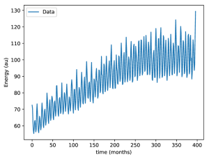
Now, let's define the parameters to use in the script. Of the 397 data points, we will use 270 for training, and the rest for testing. One particularly important parameter is lahead. This is the size of the input that our model will use to predict the next value. In this case we will use lahead = 1, which means that only one point will be used to predict the next value. This seems like an impossible task, given the complex behaviour of the energy as a function of time. The secret is that the LSTM cell has a persistent state that is able to "remember" the data that it has already seen. For a more detailed description, please read the official Keras documentation on LSTM.
[sourcecode language="bash" wraplines="false" collapse="false"]
# Set parameters
n_train = 270
lahead = 1 # time steps that the model incorporates explicitly in the input
# training parameters passed to 'model.fit(...)'
batch_size = 1
epochs = 600
[/sourcecode]
Now let's split the data into training x_train, y_train; and testing x_test, y_test. Please note that y_train is x_train shifted one place, which corresponds to univariable time-series forecasting. This method can be extended for multivariate time analysis. The same is true for x_test and y_test.
[sourcecode language="bash" wraplines="false" collapse="false"]
# Split train and validation
n_data = arr_data.shape[0]
n_valid = n_data - n_train
arr_train = arr_data[:n_train]
arr_valid = arr_data[n_train:]
# split into input and target
x_data = arr_train[:n_train-1]
y_data = arr_train[1:] # same as x_data, but with lag
reshape_3 = lambda x: x.reshape((x.shape[0], 1, 1))
x_train = reshape_3(x_data)
x_test = reshape_3(arr_valid[:-1])
reshape_2 = lambda x: x.reshape((x.shape[0], 1))
y_train = reshape_2(y_data)
y_test = reshape_2(arr_valid[1:])
[/sourcecode]
Let's build a model with one LSTM cell, that has one input and 50 outputs. These 50 outputs will be taken as inputs by one Dense layer, which gives the final 1 dimensional output of the model. Please, note the stateful = True when building the model. This allows us to play with the persistent state of the LSTM cell, otherwise the state will be reset after each call.
[sourcecode language="bash" wraplines="false" collapse="false"]
model = Sequential()
model.add(LSTM(20, input_shape=(lahead, 1), batch_size=batch_size,stateful=True))
model.add(Dense(1))
model.compile(loss='mse', optimizer='adam')
model_stateful = model
[/sourcecode]
Now we are ready to train the model!
[sourcecode language="bash" wraplines="false" collapse="false"]
for i in range(epochs):
print('iteration', i + 1, ' of ', epochs)
model_stateful.fit(x_train, y_train, batch_size=batch_size, epochs=1, validation_data=(x_test, y_test), shuffle=False)
model_stateful.reset_states()
[/sourcecode]
Of course we set the shuffle option to False, because in time series analysis the order should be kept always untouched.
To make predictions with the model, we use the predict function. Remember that the model has been reset, so first we will feed it the training data:
[sourcecode language="bash" wraplines="false" collapse="false"]
#Predict training values
predicted_stateful_train = model_stateful.predict(x_train, batch_size=batch_size)
[/sourcecode]
Now, without resetting the model, we will predict the values in the testing set. To be sure that only one input is being used to make the next time step prediction, we will do it in an explicit fashion:
[sourcecode language="bash" wraplines="false" collapse="false"]
#Predict test values one by one:
pred_test = []
for i in range(x_test.shape[0]):
# Note that only one value x_test[i] is passed as input to the model to make a prediction!
pred_test.append(model_stateful.predict(x_test[i].reshape(1,1,1), batch_size=batch_size))
#Convert list to numpy array
pred_test_1 = np.array(pred_test)
[/sourcecode]
Finally, let's se how the prediction compares with the actual data:
[sourcecode language="bash" wraplines="false" collapse="false"]
#Plot
plt.plot(y_test.reshape(-1),label= 'Data')
plt.plot(pred_test_1.reshape(-1),label= 'Forecast one-by-one')
plt.xlabel('time (months)')
plt.ylabel('Energy (au)')
plt.legend()
plt.show()
[/sourcecode]
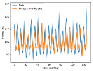
The alignment looks pretty good for a model with one input and such complex behaviour. Now, just to play around a little bit with the stateful model: what happens if we make predictions on the test set, without feeding the training data first? In order to do that, we just need to reset the model, and make predictions directly with the x_test data.
[sourcecode language="bash" wraplines="false" collapse="false"]
model_stateful.reset_states()
# Make predictions after model reset
pred_test_0 = []
for i in range(x_test.shape[0]):
pred_test_0.append(model_stateful.predict(x_test[i].reshape(1,1,1), batch_size=batch_size))
pred_test_0 = np.array(pred_test_0)
plt.plot(y_test.reshape(-1),label= 'Data')
plt.plot(y_test.reshape(-1),label= 'Data')
plt.plot(pred_test_1.reshape(-1),label= 'Forecast')
plt.plot(pred_test_0.reshape(-1),label= 'Forecast reset')
plt.xlabel('time (months)')
plt.ylabel('Energy (au)')
plt.legend()
plt.show()
[/sourcecode]
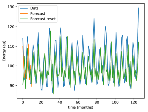
Here is what is happening: the forecast of the reset model (green curve) has a poor performance at the beginning, since it has no previous values to determine the next ones. As the reset model sees mode data, the forecast is on par with the non-reset model (orange) and is able to catch up and make a reasonable forecast compared with the actual data (blue).
+43 (0) 2622 93022-0
office@cybertec.at