October 2014

PostgreSQL has offered support for powerful analytics and window functions for a couple of years now. Many people all around the globe use analytics to make their applications more powerful and even faster. However, there is a small little feature in the area of analytics which is not that widely known. The power to use composite data types along with analytics.

A simple example

AS always some sample data is needed. For analytics we at CYBERTEC rely on a basic data set containing some data from the oil industry. Here is how it can be loaded:

test=# CREATE TABLE t_oil (country text, year int, production int);
CREATE TABLE

test=# COPY t_oil FROM PROGRAM 'curl www.cybertec.at/secret/oil.txt';
COPY 92

test=# CREATE TABLE t_oil (country text, year int, production int);

CREATE TABLE

test=# COPY t_oil FROM PROGRAM 'curl www.cybertec.at/secret/oil.txt';

COPY 92

All the data is drawn from the net (in case you got "curl" installed) and ends up in a table:

test=# SELECT *
       FROM       t_oil
       WHERE      country = 'USA'
       ORDER BY year;

 country | year | production
---------+------+------------
 USA     | 1965 |       9014
 USA     | 1966 |       9579
 USA     | 1967 |      10219
 USA     | 1968 |      10600
 USA     | 1969 |      10828
*snip*

test=# SELECT *

FROM t_oil

WHERE country = 'USA'

ORDER BY year;

country | year | production

---------+------+------------

USA | 1965 | 9014

USA | 1966 | 9579

USA | 1967 | 10219

USA | 1968 | 10600

USA | 1969 | 10828

*snip*

lag is a popular window function allowing us to move data around within the result set. lag(production, 1) means that the value in the production column should be pushed one row further down.

Here is how it works:

test=# SELECT *, lag(production, 1)
                        OVER (ORDER BY year)
            FROM            t_oil
            WHERE          country = 'USA'
            ORDER BY year;

 country | year | production |  lag 
---------+------+------------+-------
 USA     | 1965 |       9014 |     
 USA     | 1966 |       9579 |  9014
 USA     | 1967 |      10219 |  9579
 USA     | 1968 |      10600 | 10219
 USA     | 1969 |      10828 | 10600

test=# SELECT *, lag(production, 1)

OVER (ORDER BY year)

FROM t_oil

WHERE country = 'USA'

ORDER BY year;

country | year | production | lag

---------+------+------------+-------

USA | 1965 | 9014 |

USA | 1966 | 9579 | 9014

USA | 1967 | 10219 | 9579

USA | 1968 | 10600 | 10219

USA | 1969 | 10828 | 10600

Mind that we need an ORDER BY inside the OVER clause to make sure that we know into which direction to move the data. Order is essential to this kind of operation.

Moving beyond a simple field

So far so good. In the previous example one value was pushed one line down the resultset. However, it is also possible to move more complex structures around. It can be pretty useful to move an entire row:

test=# SELECT *, lag(t_oil, 1)
                        OVER (ORDER BY year)
            FROM            t_oil
            WHERE          country = 'USA'
            ORDER BY year;

 country | year | production |       lag       
---------+------+------------+------------------
 USA     | 1965 |       9014 |
 USA     | 1966 |       9579 | (USA,1965,9014)
 USA     | 1967 |      10219 | (USA,1966,9579)
 USA     | 1968 |      10600 | (USA,1967,10219)
 USA     | 1969 |      10828 | (USA,1968,10600)

test=# SELECT *, lag(t_oil, 1)

OVER (ORDER BY year)

FROM t_oil

WHERE country = 'USA'

ORDER BY year;

country | year | production | lag

---------+------+------------+------------------

USA | 1965 | 9014 |

USA | 1966 | 9579 | (USA,1965,9014)

USA | 1967 | 10219 | (USA,1966,9579)

USA | 1968 | 10600 | (USA,1967,10219)

USA | 1969 | 10828 | (USA,1968,10600)

In PostgreSQL every table definition can be seen as a composite data type. Therefore it can actually be used as a field. In this example all it does is saving us from a typing exercise. However, it can be useful if more complicated values have to be passed around (many of them).

The main question arising now is: How can a composite type be broken up again? The trick can be achieved like this:

test=# SELECT country, year, production, (lag).*  
            FROM ( SELECT *, lag(t_oil, 1) OVER (ORDER BY year)                                                                                  FROM    t_oil
                                   WHERE   country = 'USA'
                                   ORDER BY year ) AS x;

 country | year | production | country | year | production
---------+------+------------+---------+------+------------
 USA     | 1965 |       9014 |         |      |          
 USA     | 1966 |       9579 | USA     | 1965 |       9014
 USA     | 1967 |      10219 | USA     | 1966 |       9579
 USA     | 1968 |      10600 | USA     | 1967 |      10219
 USA     | 1969 |      10828 | USA     | 1968 |      10600

test=# SELECT country, year, production, (lag).*

FROM ( SELECT *, lag(t_oil, 1) OVER (ORDER BY year) FROM t_oil

WHERE country = 'USA'

ORDER BY year ) AS x;

---------+------+------------+---------+------+------------

USA | 1965 | 9014 | | |

USA | 1966 | 9579 | USA | 1965 | 9014

USA | 1967 | 10219 | USA | 1966 | 9579

USA | 1968 | 10600 | USA | 1967 | 10219

USA | 1969 | 10828 | USA | 1968 | 10600

(column).* helps us to extract all fields out of the composite type once again.

In order to receive regular updates on important changes in PostgreSQL, subscribe to our newsletter, or follow us on Facebook or LinkedIn.

Up until now, it was only possible to replicate entire database instances from one node to the other. A standby always had to consume the entire transaction log created by the primary turning the standby into a binary copy.
However, this is not always desirable. In many cases, it's necessary to split the database instance and replicate data to two different places. Just imagine having a server storing data for Europe in one and data for the US in some other database. You might not want to replicate all the data to your standbys. The standby located in Europe should only have European data and the US standby should only contain data for the United States. As mentioned before vanilla-PostgreSQL cannot do that.

walbouncer (made by CYBERTEC) can step in and fill the gap. By filtering the transaction log, it is possible to replicate only the data needed in one place. Walbouncer will act as a WAL proxy for PostgreSQL and take care of all the filtering. Here is an image showing how things work:

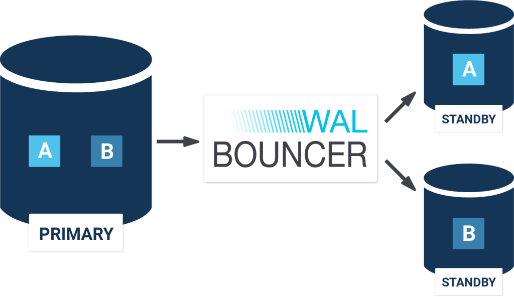
walbouncer is directly connected to the WAL stream of the primary and decides, based on its config, what to replicate to which host. This makes life very easy.

How it works

Internally the WAL is based on so called wal-records. wal-records are available for different types of operations: btree changes, COMMIT, etc. In addition to useful WAL records, PostgreSQL provides dummy records. Those records are mainly for testing but can also be used to filter WAL. Transaction log, which is meant to be left out, will be replayed with dummy records of the same length by the walbouncer. This way only the data destined for a certain server will actually reach it.

walbouncer is capable of serving many standbys at a time with very little overhead. Internally it forks for every standby and thus offers a robust system architecture. To the end user walbouncer is totally transparent - it simply acts as a proxy - and all the configuration of PostgreSQL stays the same.

Configuring walbouncer

Configuring walbouncer is simple. At this stage a simple YAML file is used to tell the system what to do. Here is an example:

listen_port: 5433
primary:
    host: localhost
    port: 5432
configurations:
    - standby1:
        match:
            application_name: standby1
        filter:
            include_tablespaces: [spc_standby1]
            exclude_databases: [test]
    - standby2:
        match:
            application_name: standby2
        filter:
            include_tablespaces: [spc_standby2]

listen_port: 5433

primary:

host: localhost

port: 5432

configurations:

- standby1:

match:

application_name: standby1

filter:

include_tablespaces: [spc_standby1]

exclude_databases: [test]

- standby2:

match:

application_name: standby2

filter:

include_tablespaces: [spc_standby2]

First of all the port the walbouncer is listening to is defined. Then all it needs are the hostname and the port to connect to the primary. Finally there is one section for each standby. In the “match” section an application name can be defined (needed for synchronous replication). In addition to that there is a “filter” section, which tells the system, what to include respectively what to leave out.

Find more information and download walbouncer here: CYBERTEC walbouncer

In case you need any assistance, please feel free to contact us.

In order to receive regular updates on important changes in PostgreSQL, subscribe to our newsletter, or follow us on Facebook or LinkedIn.

After being on the road to do PostgreSQL consulting for CYBERTEC for over a decade I noticed that there are a couple of ways to kill indexing entirely. One of the most favored ways is to apply functions or expressions on the column people want to filter on. It is a sure way to kill indexing entirely.

To help people facing this problem I decided to compile a small blog post addressing this issue. Maybe it is helpful to some of you out there.

Generating some sample data

To prove my point here is some sample data:

test=# CREATE TABLE t_time AS
            SELECT         *
            FROM            generate_series('2014-01-01', '2014-05-01', '1 second'::interval) 
AS t;
SELECT 10364401

test=# CREATE TABLE t_time AS

SELECT *

FROM generate_series('2014-01-01', '2014-05-01', '1 second'::interval)

AS t;

SELECT 10364401

The script generates a list of around 10 million rows. A list lasting from January 2014 to May 1st, 2014 is generated (one entry per second). Note that generate_series will create a list of timestamps here. To find data quickly an index will be useful:

test=# CREATE INDEX idx_t ON t_time (t);
CREATE INDEX

test=# ANALYZE;
ANALYZE

test=# CREATE INDEX idx_t ON t_time (t);

CREATE INDEX

test=# ANALYZE;

ANALYZE

Checking indexing

Under normal conditions the index shows its value as soon as a proper WHERE clause is included in our statement:

test=# explain SELECT *
            FROM       t_time
            WHERE      t >= '2014-03-03'
                       AND t < '2014-03-04';
                                          QUERY PLAN                                                              
-----------------------------------------------------------------------------------
 Index Only Scan using idx_t on t_time  (cost=0.43..3074.74 rows=86765 width=8)
   Index Cond: ((t >= '2014-03-03 00:00:00+01'::timestamp with time zone)
            AND (t < '2014-03-04 00:00:00+01'::timestamp with time zone))
 Planning time: 0.083 ms

(3 rows)

test=# explain SELECT *

FROM t_time

WHERE t >= '2014-03-03'

AND t < '2014-03-04';

QUERY PLAN

-----------------------------------------------------------------------------------

Index Only Scan using idx_t on t_time (cost=0.43..3074.74 rows=86765 width=8)

Index Cond: ((t >= '2014-03-03 00:00:00+01'::timestamp with time zone)

AND (t < '2014-03-04 00:00:00+01'::timestamp with time zone))

Planning time: 0.083 ms

(3 rows)

However, in many cases people tend to transform the left side of the comparison when searching for data. In case of large data set this has disastrous consequences and performance will suffer badly. Here is what happens:

test=# explain SELECT * FROM t_time
            WHERE          t::date = '2013-03-03';

                          QUERY PLAN                           
---------------------------------------------------------------
 Seq Scan on t_time  (cost=0.00..201326.05 rows=51822 width=8)
   Filter: ((t)::date = '2013-03-03'::date)

 Planning time: 0.090 ms

(3 rows)

test=# explain SELECT * FROM t_time

WHERE t::date = '2013-03-03';

QUERY PLAN

---------------------------------------------------------------

Seq Scan on t_time (cost=0.00..201326.05 rows=51822 width=8)

Filter: ((t)::date = '2013-03-03'::date)

Planning time: 0.090 ms

(3 rows)

PostgreSQL does not transform the WHERE-clause into a range and therefore the index is not considered to be usable. To many PostgreSQL based applications this is more or less a death sentence when it comes to performance. A handful of inefficient sequential scans can ruin the performance of the entire application easily.

In order to receive regular updates on important changes in PostgreSQL, subscribe to our newsletter, or follow us on Facebook or LinkedIn.