When people are talking about database performance monitoring, they usually think of inspecting one PostgreSQL database server at a time. While this is certainly useful, it can also be quite beneficial to inspect the status of an entire database cluster or to inspect a set of servers working together at once. Fortunately, there are easy means to achieve that with PostgreSQL. How this works can be outlined in this post.

pg_stat_statements: The best tool to monitor PostgreSQL performance in a cluster

If you want to take a deep look at PostgreSQL performance, there is really no way around pg_stat_statements. It offers a lot of information and is really easy to use.

To install pg_stat_statements, the following steps are necessary:

• run “CREATE EXTENSION pg_stat_statements” in your desired database
• add the following line to postgresql.conf: shared_preload_libraries = ‘pg_stat_statements’
• restart PostgreSQL

Once this is done, PostgreSQL will already be busy collecting data on your database hosts. However, how can we create a “clusterwide pg_stat_statements” view so that we can inspect an entire set of servers at once?

Using pg_stat_statements to check an entire database cluster

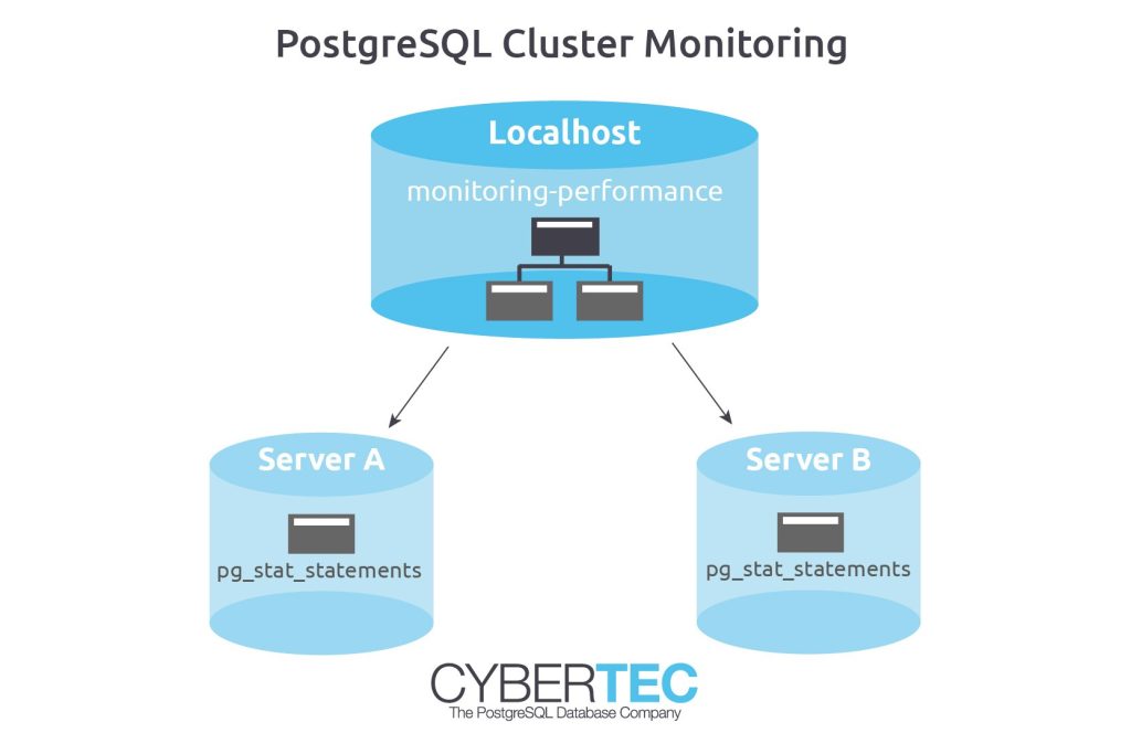
Our goal is to show data from a list of servers in a single view. One way to do that is to make use of PostgreSQL’s foreign data wrapper infrastructure. We can simply connect to all servers in the cluster and unify the data in a single view.

Let us assume we have 3 servers, a local machine, “a_server”, and “b_server”. Let us get started by connecting to the local server to run the following commands:

In the first step I created a simple user to do the database monitoring. Of course you can handle users and so on differently, but it seems like an attractive idea to use a special user for that purpose.

The next command enables the postgres_fdw extension, which is necessary to connect to those remote servers we want to access:

Then we can already create “foreign servers”.

Here is how those servers can be created:

Just replace the hostnames and the database names with your data and run those commands. The next step is already about user mapping: It might easily happen that local users are not present on the other side, so it is necessary to create some sort of mapping between local and remote users:

In this case we will login as user “postgres”. Now that two servers and the user mappings are ready, we can import the remote schema into a local schema:

For each schema there will be a separate schema. This makes it very easy to drop things again and to handle various incarnations of the same data structure.

Wiring things together

The last thing to do in our main database, is to connect those remote tables with our local data. The easiest way to achieve that is to use a simple view:

The view will simply unify all the data and add an additional column at the beginning.

Our system is now ready to use, and we can already start to run useful analysis:

The query will return all the raw data and add some percentage numbers on top of this data.

If you are interested in further information on pg_state_statements consider reading the following blog post too: https://www.cybertec-postgresql.com/en/pg_stat_statements-the-way-i-like-it/

 

---

In order to receive regular updates on important changes in PostgreSQL, subscribe to our newsletter, or follow us on Twitter, Facebook, or LinkedIn.

 

We all know that you have to pay a price for a new index you create — data modifying operations will become slower, and indexes use disk space. That's why you try to have no more indexes than you actually need.

But most people think that SELECT performance will never suffer from a new index. The worst that can happen is that the new index is not used.

However, this is not always true, as I have seen more than once in the field. I'll show you such a case and tell you what you can do about it.

An example

We will experiment with this table:

We want to find the first twenty interesting rows in category 42:

This performs fine:

PostgreSQL uses the index to find the 1000 rows with category 42, filters out the ones that are not interesting, sorts them and returns the top 20. 5 milliseconds is fine.

A new index makes things go sour

Now we add an index that can help us with sorting. That is definitely interesting if we often have to find the top 20 results:

And suddenly, things are looking worse:

What happened?

PostgreSQL thinks that it will be faster if it examines the rows in sort order using the index until it has found 20 matches. But it doesn't know how the matching rows are distributed with respect to the sort order, so it is not aware that it will have to scan 69042 rows until it has found its 20 matches (see Rows Removed by Filter: 69022 in the above execution plan).

What can we do to get the better plan?

PostgreSQL v10 has added extended statistics to track how the values in different columns are correlated, but that does not track the distributions of the values, so it will not help us here.

There are two workarounds:

1. Drop the index that misleads PostgreSQL. If that is possible, it is a simple solution. But usually one cannot do that, because the index is either used to enforce a unique constraint, or it is needed by other queries that benefit from it.
2. Rewrite the query so that PostgreSQL cannot use the offending index. Of the many possible solutions for this, I want to present two:
   • A subquery with OFFSET 0:
     PgSQL

     SELECT * FROM (SELECT * FROM skewed WHERE interesting AND category = 42 OFFSET 0) q ORDER BY sort LIMIT 20;

     1 2 3 4 5 6

     SELECT * FROM (SELECT * FROM skewed       WHERE interesting AND category = 42       OFFSET 0) q ORDER BY sort LIMIT 20;

     This makes use of the fact that OFFSET and LIMIT prevent a subquery from being “flattened”, even if they have no effect on the query result.

   • Using an expression as sort key:
     PgSQL

     SELECT * FROM skewed WHERE interesting AND category = 42 ORDER BY sort + 0 LIMIT 20;

     1 2 3 4

     SELECT * FROM skewed WHERE interesting AND category = 42 ORDER BY sort + 0 LIMIT 20;

     This makes use of the fact that PostgreSQL cannot deduce that sort + 0 is the same as sort. Remember that PostgreSQL is extensible, and you can define your own + operator!

 

---

In order to receive regular updates on important changes in PostgreSQL, subscribe to our newsletter, or follow us on Twitter, Facebook, or LinkedIn.

By Kaarel Moppel - In my last post I described what to expect from simple PL/pgSQL triggers in performance degradation sense, when doing some inspection/changing on the incoming row data. The conclusion for the most common “audit fields” type of use case was that we should not worry about it too much and just create those triggers. But in which use cases would it make sense to start worrying a bit?

So, to get more insights I conjured up some more complex trigger use cases and again measured transaction latencies on them for an extended period of time. Please read on for some extra info on the performed tests or just jump to the concluding results table at end of article.

Default pgbench vs audit triggers for all updated tables

This was the initial test that I ran for the original blog post - default pgbench transactions, with schema slightly modified to include 2 auditing columns for all tables being updated, doing 3 updates, 1 select, 1 insert (see here to see how the default transaction looks like) vs PL/PgSQL audit triggers on all 3 tables getting updates. The triggers will just set the last modification timestamp to current time and username to current user, if not already specified in the incoming row.
Results: 1.173ms vs 1.178ms i.e. <1% penalty for the version with triggers.

Single row update use case

With multi statement transactions a lot of time is actually spent on communication over the network. To get rid of that the next test consisted of just a single update on the pgbench_accounts table (again 2 audit columns added to the schema). And then again the same with an PL/pgSQL auditing trigger enabled that sets the modification timestamp and username if left empty.
Results: 0.390ms vs 0.405ms ~ 4% penalty for the trigger version. Already a bit visible, but still quite dismissible I believe.

Single row update with a trigger written in C

But what it the above 4% performance degradation is not acceptable and it sums up if we are actually touching a dozen of tables (ca 60% hit)? Can we somehow shave off some microseconds?
Well one could try to write triggers in the Postgres native language of “C”! As well with optimizing normal functions it should help with triggers. But hughh, “C” you think...sounds daunting? Well...sure, it’s not going to be all fun and play, but there a quite a lot of examples actually included in the Postgres source code to get going, see here for example.

So after some tinkering around (I'm more of a Python / Go guy) I arrived at these numbers: 0.405ms for PL/pgSQL trigger vs 0.401ms for the “C” version meaning only ~ +1% speedup! So in short – absolutely not worth the time for such simple trigger functionality. But why so little speedup against an interpreted PL language you might wonder? Yes, PL/pgSQL is kind of an interpreted language, but with a good property that execution plans and resulting prepared statements actually stay cached within one session. So if we’d use pgbench in "re-connect" mode I’m pretty sure we’d see some very different numbers.

See here for my full “C” code.

Single row update with a trigger doing “logging insert”

Here things get a bit incomparable actually as we’re adding some new data, which is not there in the “un-triggered” version. So basically I was doing from the trigger the same as the insert portion (into pgbench_history) from the default pgbench transaction. Important to note though - although were seeing some slowdown...it’s most probably still faster that doing that insert from the user transaction as we can space couple of network bytes + the parsing (in our default pgbench case statements are always re-parsed from text vs pl/pgsql code that are parsed only once (think “prepared statements”). By the way, to test how pgbench works with prepared statements (used mostly to test max IO throughput) set the “protocol” parameter to “prepared“.
Results - 0.390ms vs 0.436ms ~ 12%. Not too bad at all given we double the amount of data!

Default pgbench vs 3 “logging insert” triggers

Here we basically double the amount of data written – all updated tables get a logging entry (including pgbench_accounts, which actually gets an insert already as part on normal transaction). Results - 1.173 vs 1.285 ~ 10%. Very tolerable penalties again – almost doubling the dataset here and only paying a fraction of the price! This again shows that actually the communication latency and transaction mechanics together with the costly but essential fsync during commit have more influence than a bit of extra data itself (given we don’t have tons of indexes on the data of course). For reference - full test script can be found here if you want to try it out yourself.

Summary table

Use Case	Latencies (ms)	Penalty per TX (%)
Pgbench default vs with audit triggers for all 3 updated tables	1.173 vs 1.178	0.4%
Single table update (pgbench_accounts) vs with 1 audit trigger	0.390 vs 0.405	3.9%
Single table update (pgbench_accounts) vs with 1 audit trigger written in “C”	0.390 vs 0.401	2.8%
Single table update vs with 1 “insert logging” trigger	0.390 vs 0.436	11.8%
Pgbench default vs with 3 “insert logging” triggers on updated tables	1.173 vs 1.285	9.6%

Bonus track - trigger trivia!

* Did you know that in Postgres one can also write DDL triggers so that you can capture/reject/log structural changes for all kinds of database objects? Most prominent use case might be checking for full table re-writes during business hours.

• Also there are “statement level” triggers that are executed only once per SQL. They’re actually the default even if you don’t specify the level. And in Postgres 10 they were also extended with the “transition tables” feature, allowing you to inspect all rows changed by the statement to possibly do some summary aggregations or validation.
• When you have many triggers on a table the execution order happens alphabetically by trigger name! Additionally in case of BEFORE and INSTEAD OF triggers, the possibly-modified row returned by each trigger becomes the input to the next trigger.
• Row level BEFORE triggers are much more “cheaper” then AFTER triggers when updating a lot of rows, as they fire immediately vs at the end of the statement in which case Postgres needs to temporarily store the row state information. Situation can usually be alleviated though with some sane WHEN conditions in trigger declarations.
• And yes, it’s possible to create for example an insert trigger that inserts again into the same table that caused the trigger to fire:) Won’t then there be an infinite loop, eating up all your disk space? Yes it would...if max_stack_depth wouldn’t kick in 😉 But of course I’d advise you to keep triggers always as simple as possible.
• For writing triggers you’re not actually tied to most popular trigger language of PL/pgSQL and abovementioned “C” - at least PL/Python and PL/Perl also support triggers, and there might be some more.
• Postgres 11 will include support for triggers on partitioned tables, allowing to declare them only once! Currently one had to define them for all sub-partitions separately.