Many of you out there using PostgreSQL streaming replication might wonder what this hot_standby_feedback parameter in postgresql.conf really does. Support customers keep asking this question, so it might be useful to share this knowledge with a broader audience of PostgreSQL users out there.
VACUUM is an essential command in PostgreSQL its goal is to clean out dead rows, which are not needed by anyone anymore. The idea is to reuse space inside a table later as new data comes in. The important thing is: The purpose of VACUUM is to reuse space inside a table - this does not necessarily imply that a relation will shrink. Also: Keep in mind that VACUUM can only clean out dead rows, if they are not need anymore by some other transaction running on your PostgreSQL server.
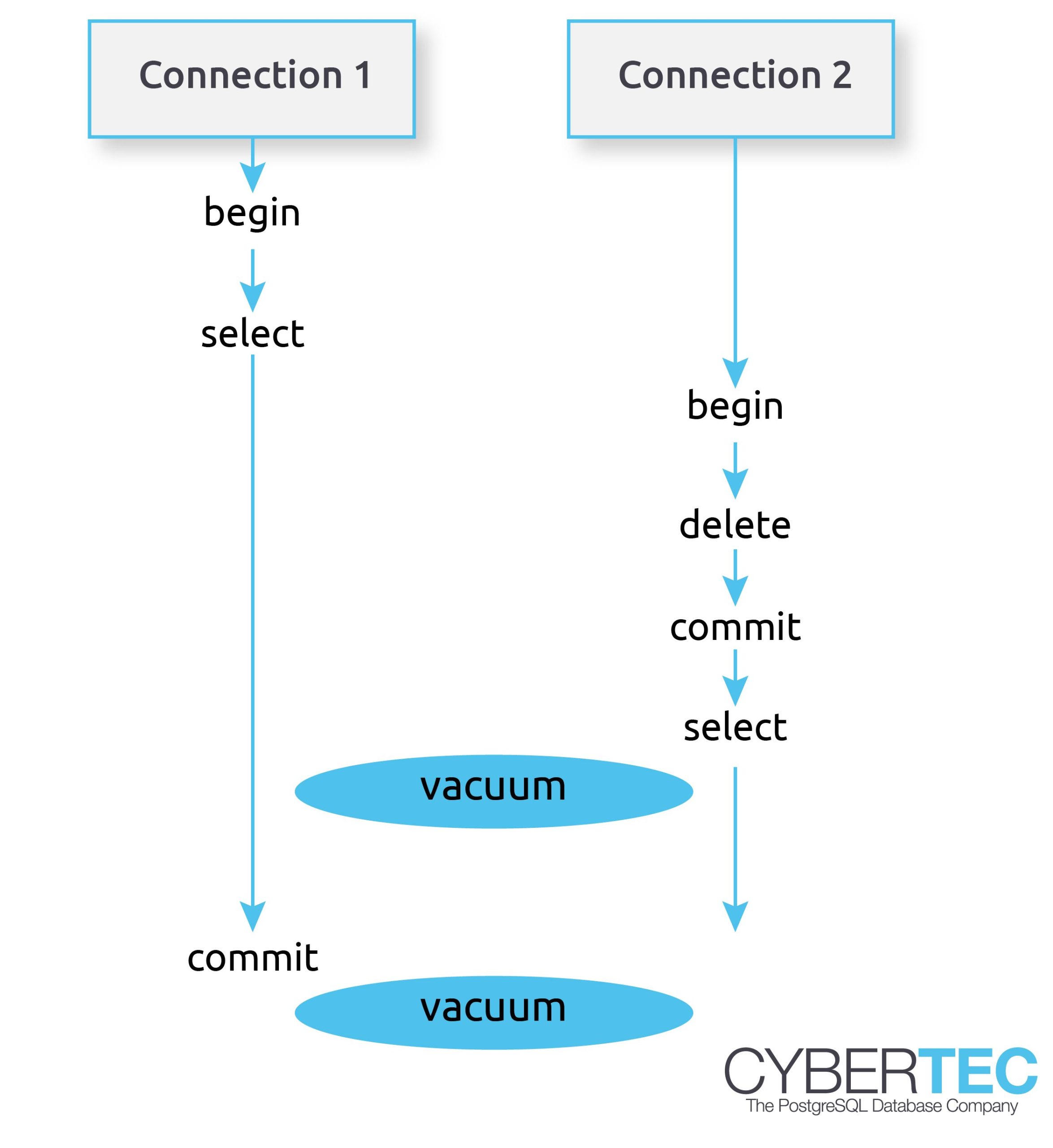
As you can see we have two connections here. The first connection on the left side is running a lengthy SELECT statement. Now keep in mind: An SQL statement will basically “freeze” its view of the data. Within an SQL statement the world does not “change” - the query will always see the same set of data regardless of changes made concurrently. That is really important to understand.
Let us take a look at the second transaction. It will delete some data and commit. The question that naturally arises is: When can PostgreSQL really delete this row from disk? DELETE itself cannot really clean the row from disk because there might still be a ROLLBACK instead of a COMMIT. In other words a rows must not be deleted on DELETE. PostgreSQL can only mark it as dead for the current transaction. As you can see other transactions might still be able to see those deleted rows.
However, even COMMIT does not have the right to really clean out the row. Remember: The transaction on the left side can still see the dead row because the SELECT statement does not change its snapshot while it is running. COMMIT is therefore too early to clean out the row.
This is when VACUUM enters the scenario. VACUUM is here to clean rows, which cannot be seen by any other transaction anymore. In my image there are two VACUUM operations going on. The first one cannot clean the dead row yet because it is still seen by the left transaction.
However, the second VACUUM can clean this row because it is not used by the reading transaction anymore.
On a single server the situation is therefore pretty clear. VACUUM can clean out rows, which are not seen anymore.
What happens in a primary/ standby scenario? The situation is slightly more complicated because how can the primary know that some strange transaction is going on one of the standbys?
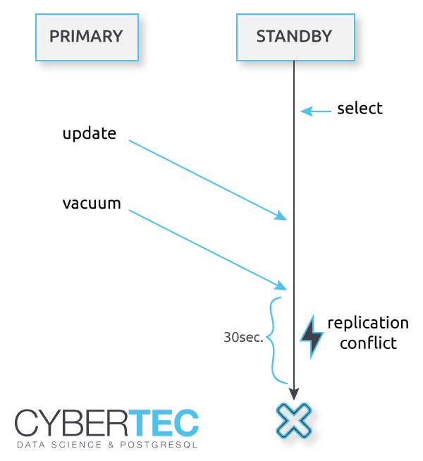
Here is an image showing a typical scenario:
In this case a SELECT statement on the replica is running for a couple of minutes. In the meantime, a change is made on the primary (UPDATE, DELETE, etc.). This is still no problem. Remember: DELETE does not really delete the row - it simply marks it as dead, but it is still visible to other transactions, which are allowed to see the “dead” row. The situation becomes critical if a VACUUM on the primary is allowed to really delete row from disk. VACUUM is allowed to do that because it has no idea that somebody on a standby is still going to need the row. The result is a replication conflict. By default a replication conflict is resolved after 30 seconds:
|
1 2 |
ERROR: canceling statement due to conflict with recovery Detail: User query might have needed to see row versions that must be removed |
If you have ever seen a message like that - it's exactly the kind of problem we are talking about here.
To solve this kind of problem, we can teach the standby to periodically inform the primary about the oldest transaction running on the standby. If the primary knows about old transactions on the standby, it can make VACUUM keep rows until the standbys are done.
This is exactly what hot_standby_feedback does. It prevents rows from being deleted too early from a standby's point of view. The idea is to inform the primary about the oldest transaction ID on the standby so that VACUUM can delay its cleanup action for certain rows.
The benefit is obvious: hot_standby_feedback will dramatically reduce the number of replication conflicts. However, there are also downsides: Remember, VACUUM will delay its cleanup operations. If the standby never terminates a query, it can lead to table bloat on the primary, which can be dangerous in the long run.
Sorting is a very important aspect of PostgreSQL performance tuning. However, improving sort performance is often misunderstood or simply overlooked by many people. So, I decided to come up with a PostgreSQL blog showing how sorts can be tuned in PostgreSQL.
To show how sorting works, I created a couple of million rows first
|
1 2 3 4 5 6 7 |
test=# CREATE TABLE t_test (x numeric); CREATE TABLE test=# INSERT INTO t_test SELECT random() FROM generate_series(1, 5000000); INSERT 0 5000000 test=# ANALYZE ; ANALYZE |
What the code does is to create a table and load 5 million random values. As you will notice, data can be loaded within seconds.
Let us try to sort the data. To keep things simple, I am using the most uncomplicated statements possible. What you can see is that PostgreSQL has to sort on disk because the data we want to sort does not fit into memory. In this case a bit more than 100 MB of data is moved to disk:
|
1 2 3 4 5 6 7 8 9 10 11 12 |
test=# explain analyze SELECT * FROM t_test ORDER BY x; QUERY PLAN -------------------------------------------------------------------------- Sort (cost=804270.42..816770.42 rows=5000000 width=11) (actual time=4503.484..6475.222 rows=5000000 loops=1) Sort Key: x Sort Method: external merge Disk: 102896kB -> Seq Scan on t_test (cost=0.00..77028.00 rows=5000000 width=11) (actual time=0.035..282.427 rows=5000000 loops=1) Planning time: 0.139 ms Execution time: 6606.637 ms (6 rows) |
Why does PostgreSQL not simply sort stuff in memory? The reason is the work_mem parameter, which is by default set to 4 MB:
|
1 2 3 4 5 |
test=# SHOW work_mem; work_mem ---------- 4MB (1 row) |
work_mem tells the server that up to 4 MB can be used per operation (per sort, grouping operation, etc.). If you sort too much data, PostgreSQL has to move the excessive amount of data to disk, which is of course slow.
Fortunately changing work_mem is simple and can even be done at the session level.
Let us change work_mem for our current session and see what happens to our example shown before.
|
1 2 |
test=# SET work_mem TO '1 GB'; SET |
The easiest way to change work_mem on the fly is to use SET. In this case I have set the parameter to 1 GB. Now PostgreSQL has enough RAM to do stuff in memory:
|
1 2 3 4 5 6 7 8 9 10 11 12 |
test=# explain analyze SELECT * FROM t_test ORDER BY x; QUERY PLAN --------------------------------------------------------------------------- Sort (cost=633365.42..645865.42 rows=5000000 width=11) (actual time=1794.953..2529.398 rows=5000000 loops=1) Sort Key: x Sort Method: quicksort Memory: 430984kB -> Seq Scan on t_test (cost=0.00..77028.00 rows=5000000 width=11) (actual time=0.075..296.167 rows=5000000 loops=1) Planning time: 0.067 ms Execution time: 2686.635 ms (6 rows) |
The performance impact is incredible. The speed has improved from 6.6 seconds to around 2.7 seconds, which is around 60% less. As you can see, PostgreSQL uses “quicksort” instead of “external merge Disk”. If you want to speed up and tune sorting in PostgreSQL, there is no way of doing that without changing work_mem. The work_mem parameter is THE most important knob you have. The cool thing is that work_mem is not only used to speed up sorts – it will also have a positive impact on aggregations and so on.
As of PostgreSQL 10 there are 3 types of sort algorithms in PostgreSQL:
“top-N heapsort” is used if you only want a couple of sorted rows. For example: The highest 10 values, the lowest 10 values and so on. “top-N heapsort” is pretty efficient and returns the desired data in almost no time:
|
1 2 3 4 5 6 7 8 9 10 11 12 13 14 |
test=# explain analyze SELECT * FROM t_test ORDER BY x LIMIT 10; QUERY PLAN ---------------------------------------------------------------------------------- Limit (cost=185076.20..185076.23 rows=10 width=11) (actual time=896.739..896.740 rows=10 loops=1) -> Sort (cost=185076.20..197576.20 rows=5000000 width=11) (actual time=896.737..896.738 rows=10 loops=1) Sort Key: x Sort Method: top-N heapsort Memory: 25kB -> Seq Scan on t_test (cost=0.00..77028.00 rows=5000000 width=11) (actual time=1.154..282.408 rows=5000000 loops=1) Planning time: 0.087 ms Execution time: 896.768 ms (7 rows) |
Wow, the query returns in less than one second.
work_mem is ideal to speed up sorts. However, in many cases it can make sense to avoid sorting in the first place. Indexes are a good way to provide the database engine with “sorted input”. In fact: A btree is somewhat similar to a sorted list.
Building indexes (btrees) will also require some sorting. Many years ago PostgreSQL used work_mem to tell the CREATE INDEX command, how much memory to use for index creation. This is not the case anymore: In modern versions of PostgreSQL the maintenance_work_mem parameter will tell DDLs how much memory to use.
Here is an example:
|
1 2 3 4 5 |
test=# timing Timing is on. test=# CREATE INDEX idx_x ON t_test (x); CREATE INDEX Time: 4648.530 ms (00:04.649) |
The default setting for maintenance_work_mem is 64 MB, but this can of course be changed:
|
1 2 3 |
test=# SET maintenance_work_mem TO '1 GB'; SET Time: 0.469 ms |
The index creation will be considerably faster with more memory:
|
1 2 3 |
test=# CREATE INDEX idx_x2 ON t_test (x); CREATE INDEX Time: 3083.661 ms (00:03.084) |
In this case CREATE INDEX can use up to 1 GB of RAM to sort the data, which is of course a lot faster than going to disk. This is especially useful if you want to create large indexes.
The query will be a lot faster if you have proper indexes in place. Here is an example:
|
1 2 3 4 5 6 7 8 9 10 11 12 |
test=# explain analyze SELECT * FROM t_test ORDER BY x LIMIT 10; QUERY PLAN -------------------------------------------------------------------------------- Limit (cost=0.43..0.95 rows=10 width=11) (actual time=0.068..0.087 rows=10 loops=1) -> Index Only Scan using idx_x2 on t_test (cost=0.43..260132.21 rows=5000000 width=11) (actual time=0.066..0.084 rows=10 loops=1) Heap Fetches: 10 Planning time: 0.130 ms Execution time: 0.119 ms (5 rows) |
In my example, the query needs far less than a millisecond. If your database happens to sort a lot of data all the time, consider using better indexes to speed things up, rather than pumping work_mem up higher and higher.
Many people out there are using tablespaces to scale I/O. By default PostgreSQL only uses a single tablespace, which can easily turn into a bottleneck. Tablespaces are a good way to provide PostgreSQL with more hardware.
Let us assume you have to sort a lot of data repeatedly: The temp_tablespaces is a parameter, which allows administrators to control the location of temporary files sent to disk. Using a separate tablespace for temporary files can also help to speed up sorting.
If you are not sure how to configure work_mem, consider checking out http://pgconfigurator.cybertec.at - it is an easy tool helping people to configure PostgreSQL.
In order to receive regular updates on important changes in PostgreSQL, subscribe to our newsletter, or follow us on Facebook or LinkedIn.
(Last updated 18.01.2023) When digging into PostgreSQL performance, it is always good to know which options one has to spot performance problems, and to figure out what is really happening on a server. Finding slow queries in PostgreSQL and pinpointing performance weak spots is therefore exactly what this post is all about.
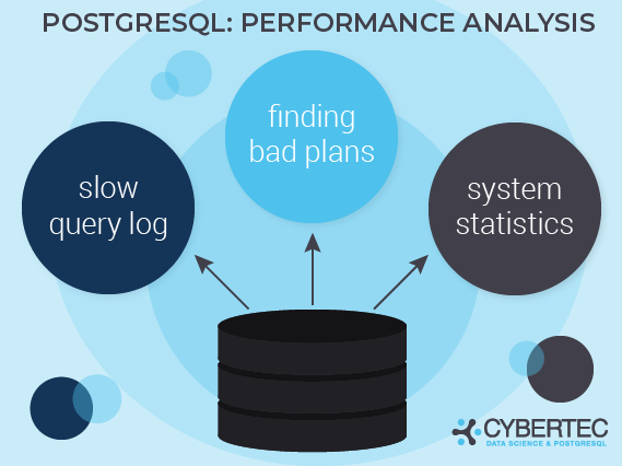
There are many ways to approach performance problems. However, three methods have proven to be really useful to quickly assess a problem. Here are my top three suggestions to handle bad performance:
Each method has its own advantages and disadvantages, which will be discussed in this document.
A more traditional way to attack slow queries is to make use of PostgreSQL's slow query log. The idea is: If a query takes longer than a certain amount of time, a line will be sent to the log. This way, slow queries can easily be spotted so that developers and administrators can quickly react and know where to look.
In a default configuration the slow query log is not active. Therefore it is necessary to turn it on. You have version choices: If you want to turn the slow query log on globally, you can change postgresql.conf:
|
1 |
log_min_duration_statement = 5000 |
If you set log_min_duration_statement in postgresql.conf to 5000, PostgreSQL will consider queries which take longer than 5 seconds to be slow queries and send them to the logfile. If you change this line in postgresql.conf there is no need for a server restart. A “reload” will be enough:
|
1 2 3 4 5 |
postgres=# SELECT pg_reload_conf(); pg_reload_conf ---------------- t (1 row) |
You can do this using an init script or simply by calling the SQL function shown above.
If you change postgresql.conf, the change will be done for the entire instance, which might be too much. In many cases you want to be a lot more precise.
Therefore it can make sense to make the change only for a certain user or for a certain database:
|
1 2 |
postgres=# ALTER DATABASE test SET log_min_duration_statement = 5000; ALTER DATABASE |
Let's reconnect and run a slow query:
|
1 2 3 4 5 6 7 |
postgres=# c test You are now connected to database 'test' as user 'hs'. test=# SELECT pg_sleep(10); pg_sleep ---------- (1 row) |
In my example I use pg_sleep to just make the system wait for 10 seconds. When we inspect the logfile, we already see the desired entry:
|
1 2 |
2018-08-20 08:19:28.151 CEST [22845] LOG: duration: 10010.353 ms statement: SELECT pg_sleep(10); |
Now you can take the statement and analyze why it is slow. A good way to do that is to run “explain analyze”, which will run the statement and provide you with an execution plan.
The advantage of the slow query log is that you can instantly inspect a slow query. Whenever something is slow, you can respond instantly to any individual query which exceeds the desired threshold. However, the strength of this approach is also its main weakness. The slow query log will track single queries. But what if bad performance is caused by a ton of not quite so slow queries? We can all agree that 10 seconds can be seen as an expensive query. But what if we are running 1 million queries which take 500 milliseconds each?
All those queries will never show up in the slow query log because they are still considered to be “fast”. What you might find, however, consists of backups, CREATE INDEX, bulk loads and so on. You might never find the root cause if you only rely on the slow query log. The purpose of the slow query log is therefore to track down individual slow statements.
The same applies to our next method. Sometimes your database is just fine, but once in a while a query goes crazy. The goal is now to find those queries and fix them. One way to do that is to make use of the auto_explain module.
The idea is similar to what the slow query log does: Whenever something is slow, create log entries. In case of auto_explain you will find the complete execution plan in the logfile - not just the query. Why does it matter?
|
1 2 3 4 5 6 7 |
test=# CREATE TABLE t_demo AS SELECT * FROM generate_series(1, 10000000) AS id; SELECT 10000000 test=# CREATE INDEX idx_id ON t_demo (id); CREATE INDEX test=# ANALYZE; ANALYZE |
The table I have just created contains 10 million rows. In addition to that an index has been defined.
|
1 2 3 4 5 6 7 8 9 10 11 12 13 14 15 16 17 |
test=# explain SELECT * FROM t_demo WHERE id < 10; QUERY PLAN --------------------------------------------------------------------------- Index Only Scan using idx_id on t_demo (cost=0.43..8.61 rows=10 width=4) Index Cond: (id < 10) (2 rows) test=# explain SELECT * FROM t_demo WHERE id < 1000000000; QUERY PLAN ------------------------------------------------------------------ Seq Scan on t_demo (cost=0.00..169248.60 rows=10000048 width=4) Filter: (id < 1000000000) JIT: Functions: 2 Inlining: false Optimization: false (6 rows) |
The queries are basically the same, but PostgreSQL will use totally different execution plans. The first query will only fetch a handful of rows and therefore go for an index scan. The second query will fetch all the data and therefore prefer a sequential scan. Although the queries appear to be similar, the runtime will be totally different. The first query will execute in a millisecond or so while the second query might very well take up to half a second or even a second (depending on hardware, load, caching and all that). The trouble now is: A million queries might be fast because the parameters are suitable - however, in some rare cases somebody might want something which leads to a bad plan or simply returns a lot of data. What can you do? Use auto_explain.
This is the idea: If a query exceeds a certain threshold, PostgreSQL can send the plan to the logfile for later inspection.
Here's an example:
|
1 2 3 4 5 6 |
test=# LOAD 'auto_explain'; LOAD test=# SET auto_explain.log_analyze TO on; SET test=# SET auto_explain.log_min_duration TO 500; SET |
The LOAD command will load the auto_explain module into a database connection. For the demo we can easily do that. In a production system you would use postgresql.conf or ALTER DATABASE / ALTER TABLE to load the module. If you want to make the change in postgresql.conf, consider adding the following line to the config file:
|
1 |
session_preload_libraries = 'auto_explain'; |
session_preload_libraries will ensure that the module is loaded into every database connection by default. There is no need for the LOAD command anymore. Once the change has been made to the configuration (don't forget to call pg_reload_conf() ) you can try to run the following query:
|
1 2 3 4 5 6 |
test=# SELECT count(*) FROM t_demo GROUP BY id % 2; count --------- 5000000 5000000 (2 rows) |
The query will need more than 500ms and therefore show up in the logfile as expected:
|
1 2 3 4 5 6 7 8 9 10 11 |
2018-08-20 09:51:59.056 CEST [23256] LOG: duration: 4280.595 ms plan: Query Text: SELECT count(*) FROM t_demo GROUP BY id % 2; GroupAggregate (cost=1605370.36..1805371.32 rows=10000048 width=12) (actual time=3667.207..4280.582 rows=2 loops=1) Group Key: ((id % 2)) -> Sort (cost=1605370.36..1630370.48 rows=10000048 width=4) (actual time=3057.351..3866.446 rows=10000000 loops=1) Sort Key: ((id % 2)) Sort Method: external merge Disk: 137000kB -> Seq Scan on t_demo (cost=0.00..169248.60 rows=10000048 width=4) (actual time=65.470..876.695 rows=10000000 loops=1) |
As you can see, a full “explain analyze” will be sent to the logfile.
The advantage of this approach is that you can have a deep look at certain slow queries and see when a query decides on a bad plan. However, it's still hard to gather overall information, because there might be millions of queries running on your system.
The third method is to use pg_stat_statements. The idea behind pg_stat_statements is to group identical queries which are just used with different parameters and aggregate runtime information in a system view.
In my personal judgement pg_stat_statements is really like a Swiss army knife. It allows you to understand what is really happening in your system.
To enable pg_stat_statements, add the following line to postgresql.conf and restart your server:
|
1 |
shared_preload_libraries = 'pg_stat_statements' |
Then run “CREATE EXTENSION pg_stat_statements” in your database.
|
1 2 3 4 5 6 7 8 9 10 11 12 13 14 15 16 17 18 19 20 21 22 23 24 25 26 27 28 29 30 31 32 33 34 35 36 37 38 39 40 41 42 43 44 45 46 47 48 49 |
test=# CREATE EXTENSION pg_stat_statements; CREATE EXTENSION test=# d pg_stat_statements View 'public.pg_stat_statements' Column | Type | Collation | Nullable | Default -----------------------+------------------+-----------+----------+--------- userid | oid | | | dbid | oid | | | toplevel | bool | | | queryid | bigint | | | query | text | | | plans | bigint | | | total_plan_time | double precision | | | min_plan_time | double precision | | | max_plan_time | double precision | | | mean_plan_time | double precision | | | stddev_plan_time | double precision | | | calls | bigint | | | total_exec_time | double precision | | | min_exec_time | double precision | | | max_exec_time | double precision | | | mean_exec_time | double precision | | | stddev_exec_time | double precision | | | rows | bigint | | | shared_blks_hit | bigint | | | shared_blks_read | bigint | | | shared_blks_dirtied | bigint | | | shared_blks_written | bigint | | | local_blks_hit | bigint | | | local_blks_read | bigint | | | local_blks_dirtied | bigint | | | local_blks_written | bigint | | | temp_blks_read | bigint | | | temp_blks_written | bigint | | | blk_read_time | double precision | | | blk_write_time | double precision | | | temp_blk_read_time | double precision | | | temp_blk_write_time | double precision | | | wal_records | bigint | | | wal_fpi | bigint | | | wal_bytes | numeric | | | jit_functions | bigint | | | jit_generation_time | double precision | | | jit_inlining_count | bigint | | | jit_inlining_time | double precision | | | jit_optimization_count | bigint | | | jit_optimization_time | double precision | | | jit_emission_count | bigint | | | jit_emission_time | double precision | | | |
The view tells you which kind of query has been executed how often, and tells you about the total runtime of this type of query as well as about the distribution of runtimes for those particular queries. The data presented by pg_stat_statements can then be analyzed. Some time ago I wrote a blog post about this issue which can be found on our website.
The advantage of this module is that you will even be able to find millions of fairly fast queries which could be the reason for a high load. In addition to that, pg_stat_statements will tell you about the I/O behavior of various types of queries. The downside is that it can be fairly hard to track down individual slow queries which are usually fast but sometimes slow.
Tracking down slow queries and bottlenecks in PostgreSQL is easy, assuming that you know which technique to use when. Use the slow query log to track down individual slow statements. auto_explain will help you to understand which slow queries are due to bad execution plans. Finally, pg_stat_statements, the Swiss army knife of PostgreSQL, will help you to understand which groups of queries might all be working together to slow your system down. This post gives you a quick overview of what's possible and what can be done to track down performance issues.
Update: see my 2021 blog post on pg_stat_statements for more detailed information on that method.
Check out Kaarel Moppel's blogpost on pg_stat_statements for a real-life example of how to fix slow queries.
From PG 12 to PG 13 the following has changed:
total_time became total_exec_time because now, there is also a total_plan_time (see table above)PostgreSQL v15 added counters for JIT (Just-In-Time compiler) statistics.
Please leave comments below. In order to receive regular updates on important changes in PostgreSQL, subscribe to our newsletter, or follow us on Facebook or LinkedIn.