The ability to run transactions is the core of every modern relational database system. The idea behind a transaction is to allow users to control the way data is written to PostgreSQL. However, a transaction is not only about writing – it is also important to understand the implications on reading data for whatever purpose (OLTP, data warehousing, etc.).

Understanding transaction isolation levels

One important aspect of transactions in PostgreSQL, and therefore in all other modern relational databases, is the ability to control when a row is visible to a user and when it is not. The ANSI SQL standard proposes 4 transaction isolation levels (READ UNCOMMITTED, READ COMMITTED, REPEATABLE READ and SERIALIZABLE) to allow users to explicitly control the behavior of the database engine. Unfortunately, the existence of transaction isolation levels is still not as widely known as it should be. Therefore I decided to blog about this topic, to give more PostgreSQL users the chance to apply this very important, yet under-appreciated feature.

The two most commonly used transaction isolation levels are READ COMMITTED and REPEATABLE READ. In PostgreSQL READ COMMITTED is the default isolation level and should be used for normal OLTP operations. In contrast to other systems, such as DB2 or Informix, PostgreSQL does not provide support for READ UNCOMMITTED, which I personally consider to be a thing of the past anyway.

What READ COMMITTED does

In READ COMMITTED mode, every SQL statement will see changes which have already been committed (e.g. new rows added to the database) by some other transactions. In other words: If you run the same SELECT statement multiple times within the same transaction, you might see different results. This is something you have to consider when writing an application.

However, within a statement the data you see is constant – it does not change. A SELECT statement (or any other statement) will not see changes committed WHILE the statement is running. Within an SQL statement, data and time are basically “frozen”.

What REPEATABLE READ does

In the case of REPEATABLE READ the situation is quite different: A transaction running in REPEATABLE READ mode will never see the effects of transactions committing concurrently – it will keep seeing the same data and offer you a consistent snapshot throughout the entire transaction. If your goal is to do reporting or if you are running some kind of data warehousing workload, REPEATABLE READ is exactly what you need, because it provides consistency. All pages of your report will see exactly the same set of data. There is no need to worry about concurrent transactions.

Transaction isolation in PostgreSQL visualized

Digging through a theoretical discussion might not be what you are looking for. So let us take a look at a picture showing graphically how things work:

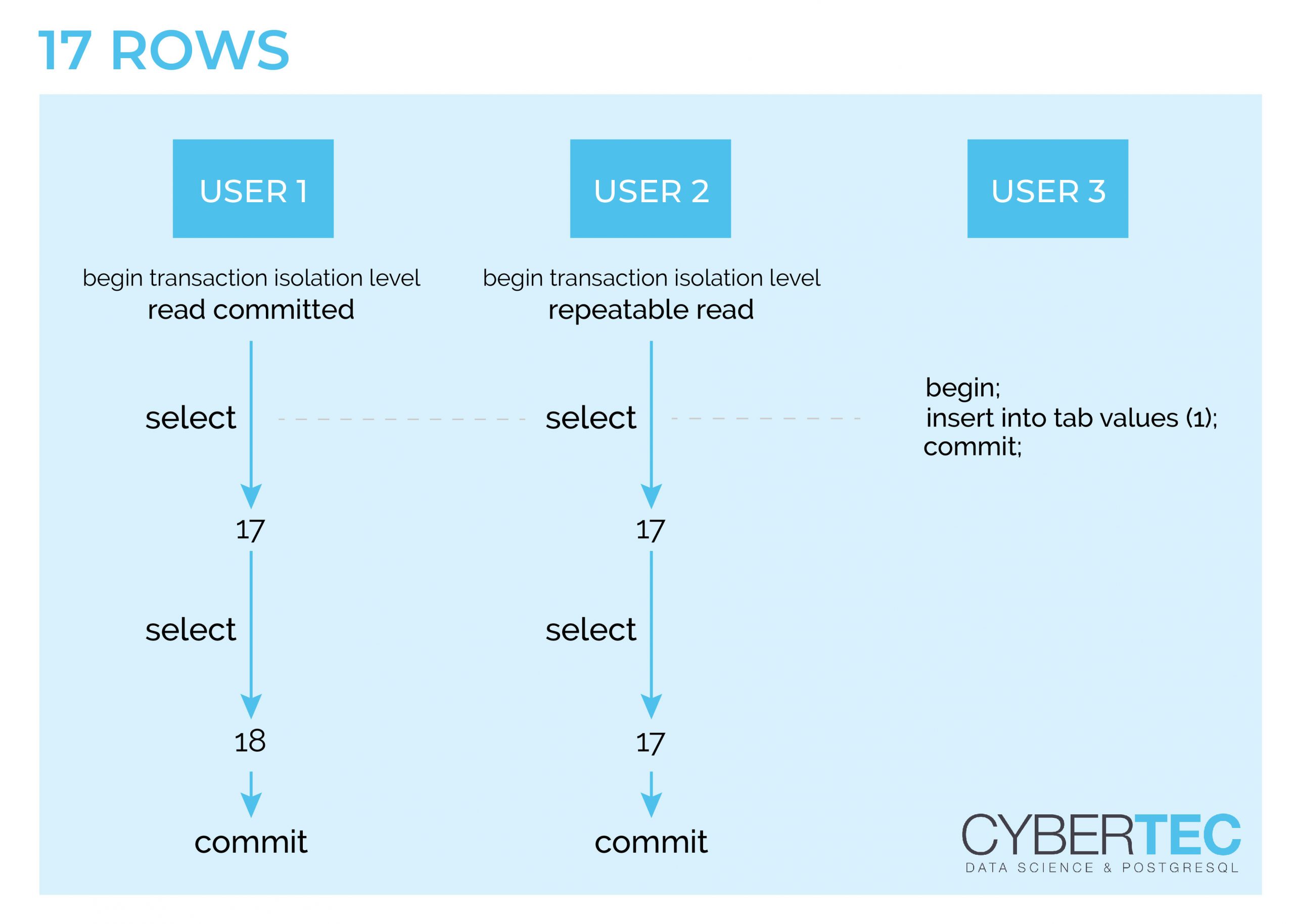
Let us assume that we have 17 rows in a table. In my example three transactions will happen concurrently. A READ COMMITTED, a REPEATABLE READ and a writing transaction. The write happens while our two reads execute their first SELECT statement. The important thing here: The data is not visible to concurrent transactions. This is a really important observation. The situation changes during the second SELECT. The REPEATABLE READ transaction will still see the same data, while the READ COMMITTED transaction will see the changed row count.

REPEATABLE READ is really important for reporting because it is the only way to get a consistent view of the data set even while it is being modified.

---

In order to receive regular updates on important changes in PostgreSQL, subscribe to our newsletter, or follow us on Facebook or LinkedIn.

If you happen to be an SQL developer, you will know that joins are really at the core of the language. Joins come in various flavors: Inner joins, left joins, full joins, natural joins, self joins, semi-joins, lateral joins, and so on. However, one of the most important distinctions is the difference between implicit and explicit joins. Over the years, flame wars have been fought over this issue. Still, not many people know what's really going on. I hope this post helps to shed some light on the situation.

Using implicit joins

Before I dig into practical examples, let's create some tables that we can later use to perform our joins:

In the next step, some rows are added to the tables:

An implicit join is the simplest way to join data. The following example shows an implicit join:

In this case, all tables are listed in the FROM clause and are later connected in the WHERE clause. In my experience, an implicit join is the most common way to connect two tables. However, my observation might be heavily biased, because an implicit join is the way I tend to write things in my daily work.

Using explicit joins

Some people prefer the explicit join syntax over implicit joins due to its readability.

The following example shows an explicit join.

In this case, tables are connected directly using an ON-clause. The ON-clause simply contains the conditions we want to use to join the tables together.

Explicit joins support two types of syntax constructs: ON-clauses and USING-clauses. An ON-clause is perfect in case you want to connect different columns with each other. A using clause is different: It has the same meaning, but it can only be used if the columns on both sides have the same name. Otherwise, a syntax error is issued:

USING is often implemented to connect keys with each other, as shown in the next example:

In my tables, both column have a column called “id”, which makes it possible to implement USING here. Keep in mind: USING is mostly syntactic sugar – there is no deeper meaning.

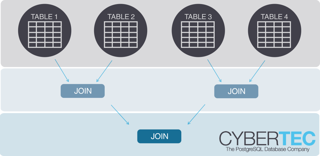
Often, an explicit join is used to join more than two tables. To show how that works, I have added another table:

Let's add some data to this table:

To perform an explicit join, just add additional JOIN and USING clauses (respectively ON clauses) to the statement.

Here's an example of an explicit join:

The same can be done with an implicit join:

However, as you can see, there is a small difference. Check the number of columns returned by the query. You will notice that the implicit join returns more. The “id” column will show up more frequently in this case, because the implicit join handles the column list in a slightly different way.

The column list is a nasty detail, because in a real application it is always better to explicitly list all columns. This little detail should be kept in mind.

join_collapse_limit: What the optimizer does

When I am on the road working as PostgreSQL consultant or PostgreSQL support guy, people often ask if there is a performance difference between implicit and explicit joins. The answer is: “Usually not”. Let's take a look at the following statement:

The explicit join produces exactly the same plan as the implicit plan shown below:

So in the majority of all cases, an implicit join does exactly the same thing as an explicit join.

join_collapse_limit

However, this is not always the case. In PostgreSQL there is a variable called join_collapse_limit:

What does it all mean? If you prefer explicit over implicit joins, the planner will always plan the first couple of joins automatically – regardless of which join order you have used inside the query. The optimizer will simply reorder joins the way they seem to be most promising. But if you keep adding joins, the ones exceeding join_collapse_limit will be planned the way you have put them into the query. As you can easily imagine, we are already talking about fairly complicated queries. Joining 9 or more tables is quite a lot and beyond the typical operation in most cases.

from_collapse_limit

There is another parameter called from_collapse_limit that does the same thing for implicit joins and has the same default value. If a query lists more than from_collapse_limit tables in its FROM clause, the ones exceeding the limit will not be re-ordered, but joined in the order they appear in the statement.

However, for the typical, “normal” query, the performance and the execution plans stay the same: it makes no difference which type of join you prefer.

If you want to read more about joins, consider reading some of our other blog posts:

• • Forcing the Join Order in PostgreSQL by Laurenz Albe
  • What is an inner join in PostgreSQL? And what is an outer join? By Hans-Jürgen Schönig
  • Understanding Lateral Joins by Hans-Jürgen Schönig

 

---

In order to receive regular updates on important changes in PostgreSQL, subscribe to our newsletter, or follow us on Facebook or LinkedIn.

By Hernan Resnizky

Machine Learning without leaving the Database - Kmeans

Every company has the opportunity to improve its decision-making process with minimal effort through the use of machine learning. However, the drawback is that for most of the DBMS, you will need to perform your Machine Learning processes outside the database. This is not the case in PostgreSQL.

As PostgreSQL contains multiple extensions to other languages. You can train and use Machine Learning algorithms without leaving PostgreSQL.

Let's take a look at how to do Kmeans, one of the most popular unsupervised learning algorithms, directly within PostgreSQL using PLPython.

KMeans in PostgreSQL Step by Step

Step 1: Load sample Data

For this example, we are going to use the iris dataset, which is publicly available. To do this, we first have to  download the data from this website to our local machine.
download the data into our local machine from

After that, you will need to create the iris table in your database:

Once the table is created, we can proceed to populate it with the data we just downloaded. Before running the following command, please delete the last empty line of iris.data

Now that we are having the data we are going to use, let's jump to kmean's core function.

Step 2: Installation of dependencies

Before creating our function, let's install the requirements:

1. Python: Follow the instructions here that correspond to the OS of the machine, where PostgreSQL is installed. Please notice that there are 2 main versions of Python currently, 2.7 and 3.5. The Python community is transitioning from one to the other, so you will need to decide to which one to stick to. The Python code presented here runs on both of them, but if you are planning to use PL/Python further in the future you should take this into account. You can also install both side by side. The only limitation is that both cannot be ran during the same session. For more information visit this link
2. PL/Python: PL/Python is the extension that allows you to run Python code without leaving Postgres. At least starting from 9.5, there are two plpython extensions available, one for python 2 (plpython) and one for python3 (plpython3). Again, you can have both installed at the same time.
3. Once you have them installed, you need to create the extension. To do so, connect to the database and type

and/or

4. Install additional Python Libraries: use your favorite Python package manager (pip, conde, etc.) and install scikit-learn and pandas. By the way, both packages are a must if you want to start digging into Machine Learning with Python

Step 3: Kmeans in PostgreSQL in a nutshell

Functions written with PL/Python can be called like any other SQL function. As Python has endless libraries for Machine Learning, the integration is very simple. Moreover, apart from giving full support to Python, PL/Python also provides a set of convenience functions to run any parametrized query. So, executing Machine Learning algorithms can be a question of a couple of lines. Let’s take a look:

As you can see, the script is very simple. Firstly, we import the functions we need, then we generate a string from the columns passed or replace it with * if an empty array is passed and then finally we build the query using PL/Python’s execute function. Although it is out of the scope of this article, I strongly recommend reading about how to parametrize queries using PL/Python.

Once the query is built and executed, we need to cast it to convert it into a data frame and transform the numeric variables into numeric type (they may be interpreted as something else by default). Then, we call kmeans, where the passed input groups amount is passed as parameter as the number of clusters you want to obtain. Finally, we dump it into a cPickle and returned the object stored in a Pickle. Pickling is necessary to restore the model later, since otherwise Python would not be able to restore the kmeans object directly from a bytearray coming from PostgreSQL.

The final line specifies the extension language: in this case, we are using python 2 and, for that reason, the extension is called plpythonu. If you would like to execute it in Python 3, you should use the extension language named plpython3u

 Step 4: Storing the Model

It doesn't make much sense to create a model and not do anything with it. So, we will need to store it.

To do so, let’s create a models table first:

In this case, our table has just a primary key and a byte array field, that is the actual model serialized. Please note that it is the same data type as the one that is returned by our defined kmeans.

Once we have the table, we can easily insert a new record with the model:

In this case, we are passing the columns parameter as an empty array to perform clustering with all the numeric variables in the table. Please consider that this is just an example. In a production case you may want to add, for example, some extra fields that can make it easier to identify the different models.

Step 5: Displaying Model Info

So far, we were able to create a model and store it but getting it directly from the database isn't very useful. You can check it by running

select * from models;

For that reason, we will need to get back to Python to display useful information about our model. This is the function we are going to use:

Let’s start from the beginning: we are passing, again, the table containing the models and the column that holds the binary. The output is read by cpickle’s load function (here you can see how results from a plpython query are loaded into Python).

Once the model is loaded, we know that all kmeans objects have an attribute “cluster_centers_” , which is where the centroids are stored. Centroids are the mean vectors for each group, i.e., the mean for each variable in each group. Natively, they are stored as a numpy array but since plpython cannot handle numpy arrays, we need to convert them to a list of lists. That is the reason why the returned object is the output of listing every row, producing a list of lists, where each sub-list represents a group’s centroid.

This is just an example of how to output a certain characteristic of a model. You can create similar functions to return other characteristics or even all together.

Let’s take a look at what it returns:

Each of the elements enclosed by braces represent a group and the values are its vector of means.

Step 6: Making Predictions

Now that we have a model, let’s use it to do predictions! In kmeans, this means passing an array of values (corresponding to each of the variables) and get the group number it belongs to. The function is very similar to the previous one:

Compared to the previous function, we add one input parameter (input_values), passing the input values representing a case (one value per variable) for which we want to get the group based on the clustering.

Instead of returning an array of floats, we return an array of integers because we are talking about a group index.

Please notice that you need to pass an array of arrays, even if you are passing only one element. This has to do with how Python handles arrays.

We can also pass column names to the function, for example:

As you can see, the associated group is strongly correlated with the species they are.

Conclusion

We have seen in this article that you can train and use machine learning without leaving Postgres. However, you need to have knowledge of Python to prepare everything. Still, this can be a very good solution to make a complete machine learning toolkit inside PostgreSQL for those that may not know how to do it in Python or any other language.

 

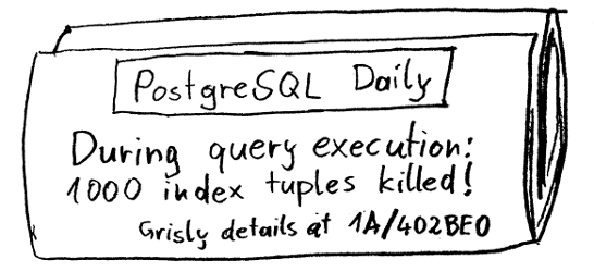
Since I only recently learned about the concept of “killed index tuples”, I thought there might be some others who are not yet familiar with this interesting PostgreSQL concept.

This may give you an explanation the next time you encounter wildly varying execution times for the same execution plan of the same PostgreSQL query.

Before we look more closely at the index, let's review the life cycle of a table row version (“heap tuple”).

Life, death and visibility in the table heap

It is widely known that the visibility of heap tuples is determined by the system columns xmin and xmax (though there is more to xmax than meets the eye). A heap tuple is “dead” if its xmax is less than the xmin of all active transactions.

Now xmin and xmax are only valid if the respective transactions have been marked committed in the “commit log”. Consequently, any transaction that needs to know if it can see a tuple has to consult the commit log. To save future readers that extra work, the first one that consults the commit log will save the information in the tuple's “hint bits”.

Dead tuples are eventually reclaimed by VACUUM.

This is all fairly well known, but how is the situation with index entries?

Life, death and visibility in the index

To avoid redundancy and to keep index tuples small, the visibility information is not stored in the index.
The status of an index tuple is determined by the heap tuple it points to, and both are removed by VACUUM at the same time.

As a consequence, an index scan has to inspect the heap tuple to determine if it can “see” an entry. This is the case even if all the columns needed are in the index tuple itself. Even worse, this “heap access” will result in random I/O, which is not very efficient on spinning disks.

This makes index scans in PostgreSQL more expensive than in other database management systems that use a different architecture. To mitigate that, several features have been introduced over the years:

• PostgreSQL 8.1 introduced the “bitmp index scan”. This scan method first creates a list of heap blocks to visit and then scans them sequentially. This not only reduces the random I/O, but also avoids that the same block is visited several times during an index scan.
• PostgreSQL 9.2 introduced the “index-only scan”, which avoids fetching the heap tuple. This requires that all the required columns are in the index and the “visibility map” shows that all tuples in the table block are visible to everybody.

But I want to focus on another feature that was also introduced in 8.1, yet never made it into the release notes.

Killed index tuples

The feature was introduced with this commit:

Whenever an index scan fetches a heap tuple only to find that it is dead (that the entire “HOT chain” of tuples is dead, to be more precise), it marks the index tuple as “killed”. Then future index scans can simply ignore it.

This “hint bit for indexes” can speed up future index scans considerably.

An example

Let's create a table to demonstrate killed index tuples. We have to disable autovacuum so that it does not spoil the effect by removing the dead tuples.

We create a number of dead tuples by deleting rows from the table:

Spot the differences!

Now we run the same query twice:

Discussion of the example

There are a number of things that cannot account for the difference:

• Often the second execution is faster because the first run has to read more data from secondary storage, which are already cached on the second run. But you can observe from the execution plan that in both cases, all blocks were already in the cache (“shared hit”) and none had to be read from disk.
• No hint bits had to be written during the first execution (no buffers were “dirtied”), because that was already done during the sequential scan from the DELETE.

What happened is that the first execution had to visit all the table blocks and killed the 799000 index tuples that pointed to dead tuples.
The second execution didn't have to do that, which is the reason why it was ten times faster.

Note that the difference in blocks touched by the two queries is not as big as one might suspect, since each table block contains many dead tuples (there is a high correlation).

It is also worth noting that even though they are not shown in the EXPLAIN output, some index pages must have been dirtied in the process, which will cause some disk writes from this read-only query.

Conclusion

Next time you encounter mysterious query run-time differences that cannot be explained by caching effects, consider killed index tuples as the cause. This may be an indication to configure autovacuum to run more often on the affected table, since that will get rid of the dead tuples and speed up the first query execution.

 

---

In order to receive regular updates on important changes in PostgreSQL, subscribe to our newsletter, or follow us on Twitter, Facebook, or LinkedIn.