Last time we imported OpenStreetMap datasets from Iceland to PostGIS. To quickly visualize our OSM data results, we will now use QGIS to render our datasets and generate some nice maps on the client.

Let’s start with our prerequisites:

1. A PostGIS enabled PostgreSQL database preloaded with OpenStreetMap datasets as described in blogpost https://www.cybertec-postgresql.com/en/open-street-map-to-postgis-the-basics/
2. An up and running QGIS Client, see https://www.qgis.org/de/site/ for further instructions
3. A Git-Client to checkout some predefined styles for QGIS

Import OSM data sets into QGIS

QGIS supports PostgreSQL/PostGIS out of the box.
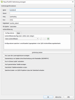
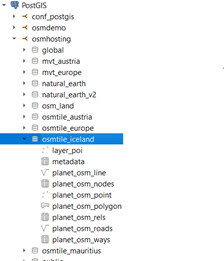
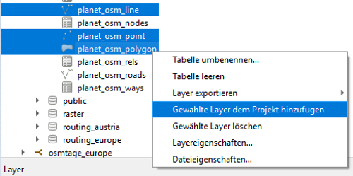
We can import our datasets by defining our database connection (1), showing up the db catalog (2) and adding datasets of interest (3) to our workspace.

Step 1	Step 2	Step 3

 

QGIS will automatically apply basic styles for the given geometry types and will start loading features of the current viewport and extent. Herby the tool will use information from PostGIS’s geometry_column view to extract geometry column, geometry type, spatial reference identifier and number of dimensions. To check what PostGIS is offering to QGIS, let’s query this view:

 

This brings up the following results:

tblname	geocol	geodim	srid	type
planet_osm_point	way	2	3857	POINT
planet_osm_line	way	2	3857	LINESTRING
planet_osm_polygon	way	2	3857	GEOMETRY
planet_osm_roads	way	2	3857	LINESTRING

 

For type geometry, QGIS uses geometrytype to finally assess geometry’s type modifier.

Basic styling of OSM data in QGIS

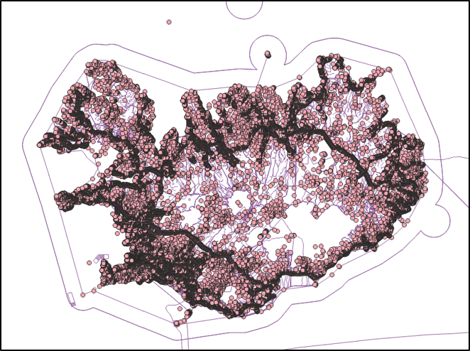
As mentioned before, QGIS applies default styles to our datasets after being added to the QGIS workspace. Figure 1 gives a first impression on how points and lines from OpenStreetMap are visualized this way.

 

It’s now up to the user the define further styling rules to turn this basic map into a readable and performant map.

As a quick reminder - we imported our osm dump utilizing osm2pgsql with a default-style and no transformations into PostGIS. This resulted in three major tables for points, lines and polygons. It’s now up to the map designer to filter out relevant objects, such as amenities represented as points within the GIS client, to apply appropriate styling rules. Alternatively, it’s a good practice to the parametrize osm2pgsql during import or set up further views to normalize the database model.

Back to our styling task - how can we turn this useless map into something useable?

Please find below some basic rules to start with:

1. Study OSM’s data-model 😊
2. Define which features are of interest and on which scale to present
3. Develop queries to grab relevant features
4. Turn queries in QGIS styling rules utilizing expressions
5. Evaluate map beauty and performance
6. Enjoy

Let me present this approach on amenities and pick some representative amenity types.

 

amenity	count
waste_basket	1346
bench	1285
parking	479
…

 

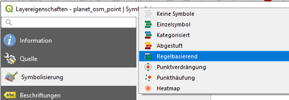
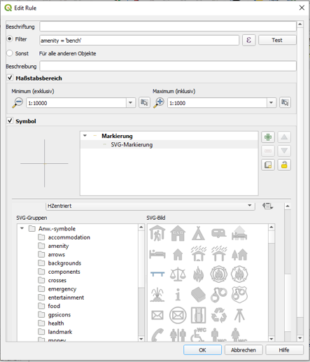
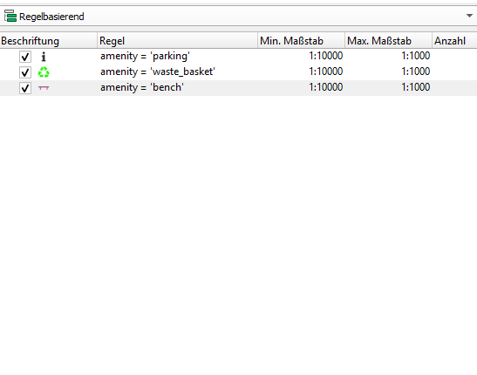
To style osm_points and apply individual styles for waste_basket, bench and parking we open up the layer properties, click on symbology and finally select rule-based styling as demonstrated in the pictures below.
For each amenity type then, we set up an individual rule by

• defining a query to select the amenity of interest,
• defining an appropriate scale and
• defining a symbol (svg marker in our case)

 

Step 1	Step 2	Step 3

 

After zooming in, your map shows your styled amenities like below.

 

 

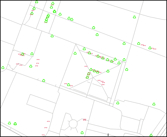
Well, better but not really appealing you might think, and you are absolutely right.
Luckily, we don’t have to start from scratch, and we can apply given styles to achieve better results.

But wait – we are not done. Let’s see what QGIS is requesting from the database to understand how actions in the map are converted to SQL statements. To do that, let’s enable LogCollector in postgres.conf and monitor the log file to grab the current sql statements. Subsequently this enables us to execute the query with explain analyse in the console to start with possible optimizations.

The resulting explain plan draws attention to a possibly useful, but missing index on column amenity, which has not been created by default by osm2pgsql. Additionally, the explain plain highlights the utilization of planet_osm_point_way_idx, an index on geometry column way, which is being used to quickly identify features, whose bounding boxes intersect with our map extent.

 

At this point it’s worth to mention auto_explain, a PostgreSQL extension which is logging execution plans for slow running queries automatically. As shortcut, checkout Kareel’s post about this great extension.

Import and apply QGIS styles

Let’s import layer settings on our datasets. For this demo I downloaded layer settings from https://github.com/yannos/Beautiful_OSM_in_QGIS, which result in a typical OpenStreetMap rendering view.

For each layer (point, line and polygon), open up the layer properties, go to symbology and load the individual layer settings file.

 

Step 1	Step 2

 

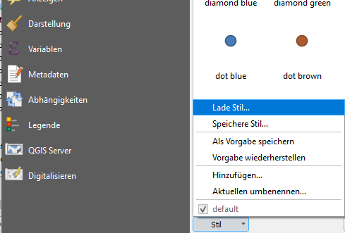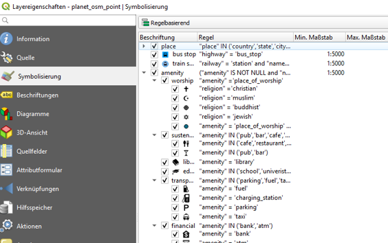Figure 3 shows the resulting map, which serves as good foundation for further adoptions.

It should be stressed that adding styling complexity is not free in terms of computational resources.
Slow loading maps on the client side are mostly caused by missing scale boundaries, expensive expressions leading to complex queries and missing indices on your backend, just to mention some of those traps.
OSM’s common style (https://www.openstreetmap.org) is generally very complex resulting in a resource-intensive rendering.

 

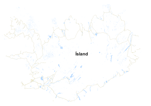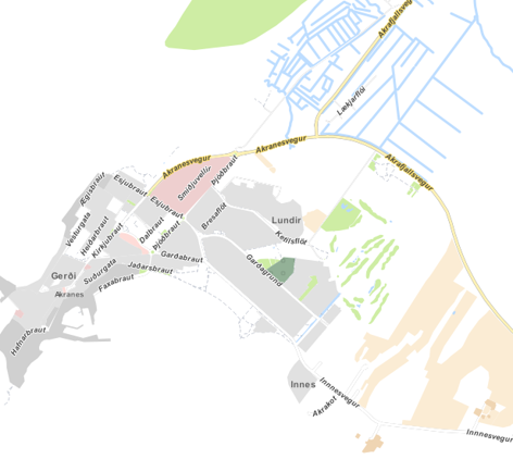Figure 3 Customized QGIS Styling Yannos, https://github.com/yannos/Beautiful_OSM_in_QGIS

Results

This time I briefly discussed how spatial data can be easily added from PostGIS to QGIS to ultimately create a simple visualization. This particular post emphasizes style complexity and finally draws attention to major pitfalls leading to slow rendering processes.

 

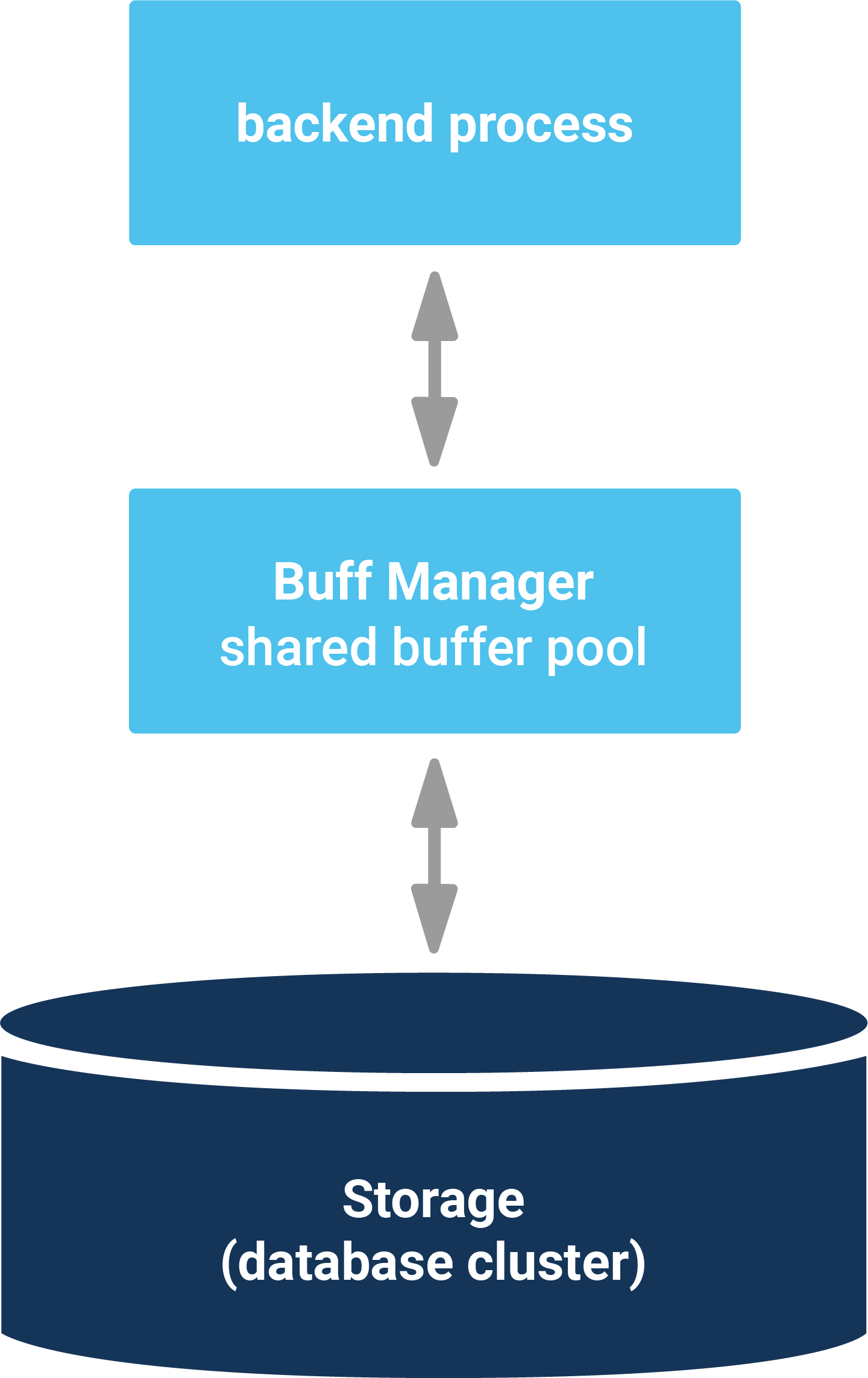
The PostgreSQL caching system has always been a bit of a miracle to many people and many have asked me during consulting or training sessions: How can I figure out what the PostgreSQL I/O cache really contains? What is in shared buffers and how can one figure out? This post will answer this kind of question and we will dive into the PostgreSQL cache.

Creating a simple sample database to illustrate shared_buffers

Before we can inspect shared_buffers, we have to create a little database:

To keep it simple I have created a standard pgbench database containing 1 million rows, as follows:

Deploying 1 million rows is pretty fast. In my case it took around 1.5 seconds (on my laptop).

Deploying pg_buffercache - shared_buffers illustration

Now that we have some data, we can install the pg_buffercache extension, which is ideal if you want to inspect the content of the PostgreSQL I/O cache:

pg_buffercache will return one row per 8k block in shared_buffers. However, to make sense out of the data one has to understand the meaning of those OIDs in the view. To make it easier for you I have created some simple example.

Let us take a look at the sample data first:

My demo database consists of 4 small tables.

Inspecting per database caching

Often the question is how much data from which database is currently cached. While this sounds simple you have to keep some details in mind:

The reldatabase column contains the object ID of the database a block belongs to. However, there is a “special” thing here: 0 does not represent a database but rather the pg_global schema. Some objects in PostgreSQL such as the list of databases, the list of tablespaces or the list of users are not stored in a database – this information is global. Therefore “0” needs some special treatment here. Otherwise, the query is pretty straightforward. To figure out how much RAM is currently not empty, we have to go and count the empty entries which have no counterpart in pg_database. In my example, the cache is not really fully populated, but mostly empty. On a real server with real data and real load, the cache is almost always 100% in use (unless your configuration is dubious).

Inspecting your current database

There is one more question many people are interested in: What does the cache know about my database? To answer that question, I will access an index to make sure some blocks will be held in shared_buffers:

The following SQL statement will calculate how many blocks from which table (r) respectively index (relkind = i) are currently cached:

We deliberately exclude all relations with object ID below 16384, because these low IDs are reserved for system objects. That way, the output only contains data for user tables.

As you can see, the majority of blocks in memory originate from pgbench_accounts. This query is therefore a nice way to instantly find out what is in cache and what is not. There is a lot more information to be extracted, but for most use cases those two queries will answer the most pressing questions.

Finally …

If you want to know more about PostgreSQL and performance in general, I suggest checking out one of our other posts in PostgreSQL performance issues, or take a look at our most recent performance blogs.

 

---

In order to receive regular updates on important changes in PostgreSQL, subscribe to our newsletter, or follow us on Twitter, Facebook, or LinkedIn.

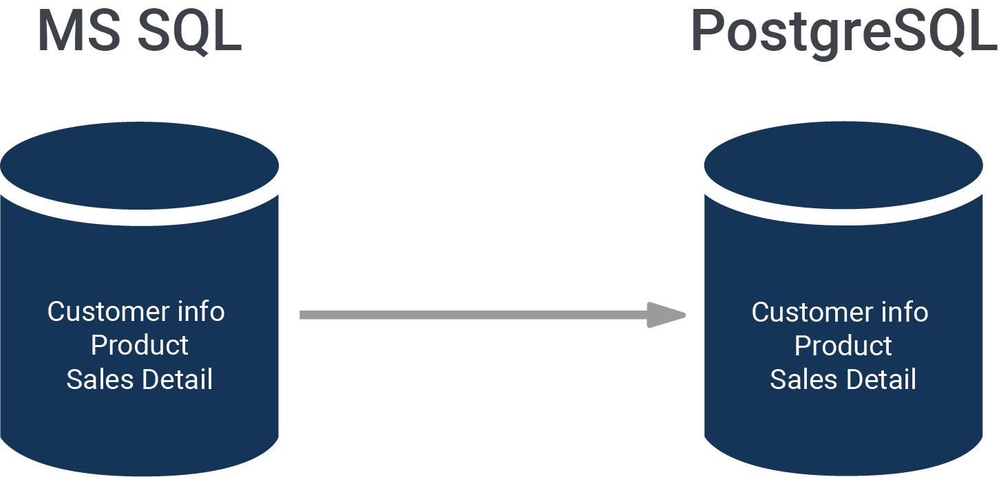
When migrating from MS SQL to PostgreSQL, one of the first things people notice is that in MS SQL, object names such as tables and columns all appear in uppercase. While that is possible on the PostgreSQL side as well it is not really that common. The question therefore is: How can we rename all those things to lowercase - easily and fast?

 

 

Finding tables to rename in PostgreSQL

The first question is: How can you find the tables which have to be renamed? In PostgreSQL, you can make use of a system view (pg_tables) which has exactly the information you need:

This query does not only return a list of tables which have to be renamed. It also creates a list of SQL commands.

If you happen to use psql directly it is possible to call ...

… directly after running the SQL above. gexec will take the result of the previous statement and consider it to be SQL which has to be executed. In short: PostgreSQL will already run the ALTER TABLE statements for you.

The commands created by the statement will display a list of instructions to rename tables:

Avoid SQL injection at all cost

However, the query I have just shown has a problem: It does not protect us against SQL injection. Consider the following table:

In this case the name of the table contains blanks. However, it could also contain more evil characters, causing security issues. Therefore it makes sense to adapt the query a bit:

The quote_ident function will properly escape the list of objects as shown in the listing below:

gexec can be used to execute this code directly.

Renaming columns in PostgreSQL to lowercase

After renaming the list of tables, you can turn your attention to fixing column names. In the previous example, I showed you how to get a list of tables from pg_tables. However, there is a second option to extract the name of an object: The regclass data type. Basically regclass is a nice way to turn an OID to a readable string.

The following query makes use of regclass to fetch the list of tables. In addition, you can fetch column information from pg_attribute:

gexec will again run the code we have just created, and fix column names.

Finally

As you can see, renaming tables and columns in PostgreSQL is easy. Moving from MS SQL to PostgreSQL is definitely possible - and tooling is more widely available nowadays than it used to be. If you want to read more about PostgreSQL, checkout our blog about moving from Oracle to PostgreSQL.

By Kevin Speyer - In this post, we will cover a step by step guide on how to implement a clustering algorithm within PostgreSQL. The clustering algorithm is the well-known k-means, which splits data into groups by minimising the sum of the squared distances of each point to the corresponding group average. This method belongs to the so called unsupervised learning algorithms, because it does not require labels to train the model. Instead, the model extracts the underlying structure by observing the distribution of data.
In a previous post we've covered how to execute a python k-means algorithm inside Postgres. In this case, we will use another library written in c, from this repository.

Set up

First, let's clone the repository into our computer:

[sourcecode language="bash" wraplines="false" collapse="false"]
$ git clone git@github.com:cybertec-postgresql/kmeans-postgresql.git
$ cd kmeans-postgresql
[/sourcecode]

Now, we have to install the package:

[sourcecode language="bash" wraplines="false" collapse="false"]
$ sudo make install
[/sourcecode]

To test the extension, I will create a new database. So let's start the PostgreSQL client:

[sourcecode language="bash" wraplines="false" collapse="false"]
$ psql -U postgres
[/sourcecode]

[sourcecode language="sql" wraplines="false" collapse="false"]
# CREATE DATABASE kmeans
[/sourcecode]

Finally, let's run the kmeans.sql script to create the functions in the database. This will allow us to run the k-means algorithm from within the database.

[sourcecode language="bash" wraplines="false" collapse="false"]
$ psql -f kmeans--1.1.0.sql -U user -d kmeans
[/sourcecode]

We are done with the setup!

Using the cluster algorithm

Now, let's test the algorithm. We can use the test data from the repository, which is located in the "data/" directory. We have to create a table to copy the data into:

[sourcecode language="bash" wraplines="false" collapse="false"]
$ psql -U user -d kmeans
[/sourcecode]

[sourcecode language="sql" wraplines="false" collapse="false"]
kmeans=> CREATE TABLE testdata(val1 float, val2 float, val3 float);
kmeans=> i input/kmeans.source
kmeans=> COPY testdata FROM './data/testdata.txt' ( FORMAT CSV, DELIMITER(' ') );
[/sourcecode]

Now, we can call the kmeans function from the database and see the results:

[sourcecode language="sql" wraplines="false" collapse="false"]
kmeans=> SELECT kmeans(ARRAY[val1, val2], 5) OVER (), val1, val2 FROM testdata limit 10;
kmeans | val1 | val2
--------+-----------+-----------
2 | 1.208985 | 0.421448
3 | 0.504542 | -0.28573
2 | 0.630568 | 1.054712
2 | 1.056364 | 0.601873
0 | 1.095326 | -1.447579
1 | -0.210165 | 0.000284
0 | -0.367151 | -1.255189
0 | 0.868013 | -1.063465
3 | 1.704441 | -0.644833
0 | 0.565619 | -1.637858
(10 rows)
[/sourcecode]

 
The last parameter (5 in this case) is the number of clusters to divide the data into. The OVER clause gives us the possibility to perform the clusterization in a window. This can be achieved using PARTITION BY, like this:

[sourcecode language="sql" wraplines="false" collapse="false"]
kmeans=> SELECT kmeans(ARRAY[val1, val2], 2) OVER (partition by val1 > 0), val1, val2 FROM testdata  limit10;
[/sourcecode]

In this case, the algorithm runs separately for all data with val1 > 0, exactly like a window function.

Visualizing the clusters

To visualize the results, we can run the perl script in the repository. If you have never used gnuplot, it is necessary to install it first:

[sourcecode language="bash" wraplines="false" collapse="false"]
$ sudo dnf install -y gnuplot
[/sourcecode]

or for APT package manager

[sourcecode language="bash" wraplines="false" collapse="false"]
$ sudo apt-get install -y gnuplot
[/sourcecode]

Lastly, run the plot script and observe the results!

[sourcecode language="bash" wraplines="false" collapse="false"] perl plot-cybertec.pl -d kmeans -k 4 [/sourcecode]

The output of the script is displayed: the algorithm divides the data into four clusters

 

If you are not working on a local machine, or just want to look at the plot in the terminal, you can add the -t option:

[sourcecode language="bash" wraplines="false" collapse="false"]

perl plot-cybertec.pl -d kmeans -k 4 -t

[/sourcecode]

And you should see something like this in the terminal: