February 2018

About sequences

Sequences are used to generate artificial numeric primary key columns for tables.
A sequence provides a “new ID” that is guaranteed to be unique, even if many database sessions are using the sequence at the same time.

Sequences are not transaction safe, because they are not supposed to block the caller. That is not a shortcoming, but intentional.

As a consequence, a transaction that requests a new value from the sequence and then rolls back will leave a “gap” in the values committed to the database. In the rare case that you really need a “gap-less” series of values, a sequence is not the right solution for you.

PostgreSQL's traditional way of using sequences (nextval('my_seq')) differs from the SQL standard, which uses NEXT VALUE FOR .

New developments in PostgreSQL v10

Identity columns

PostgreSQL v10 has introduced the standard SQL way of defining a table with an automatically generated unique value:

GENERATED { ALWAYS | BY DEFAULT } AS IDENTITY [ ( sequence_options ) ]

1	GENERATED { ALWAYS \| BY DEFAULT } AS IDENTITY [ ( sequence_options ) ]

Here is an example:

CREATE TABLE my_tab (
   id bigint GENERATED BY DEFAULT AS IDENTITY PRIMARY KEY,
   ...
);

CREATE TABLE my_tab (

id bigint GENERATED BY DEFAULT AS IDENTITY PRIMARY KEY,

...

);

Behind the scenes, this uses a sequence, and it is roughly equivalent to the traditional

CREATE TABLE my_tab (
   id bigserial PRIMARY KEY,
   ...
);

CREATE TABLE my_tab (

id bigserial PRIMARY KEY,

...

);

which is a shorthand for

CREATE SEQUENCE my_tab_id_seq;

CREATE TABLE my_tab (
   id bigint PRIMARY KEY DEFAULT nextval('my_tab_id_seq'::regclass),
   ...
);

ALTER SEQUENCE my_tab_id_seq OWNED BY my_tab.id;

CREATE SEQUENCE my_tab_id_seq;

CREATE TABLE my_tab (

id bigint PRIMARY KEY DEFAULT nextval('my_tab_id_seq'::regclass),

...

);

ALTER SEQUENCE my_tab_id_seq OWNED BY my_tab.id;

The problem with such a primary key column is that the generated value is a default value, so if the user explicitly inserts a different value into this column, it will override the generated one.

This is usually not what you want, because it will lead to a constraint violation error as soon as the sequence counter reaches the same value. Rather, you want the explicit insertion to fail, since it is probably a mistake.

For this you use GENERATED ALWAYS:

CREATE TABLE my_tab (
   id bigint GENERATED ALWAYS AS IDENTITY PRIMARY KEY,
   ...
);

CREATE TABLE my_tab (

id bigint GENERATED ALWAYS AS IDENTITY PRIMARY KEY,

...

);

You can still override the generated value, but you'll have to use the OVERRIDING SYSTEM VALUE clause for that, which makes it much harder for such an INSERT to happen by mistake:

INSERT INTO my_tab (id) OVERRIDING SYSTEM VALUE VALUES (42);

1	INSERT INTO my_tab (id) OVERRIDING SYSTEM VALUE VALUES (42);

New system catalog `pg_sequence`

Before PostgreSQL v10, Postgres stored a sequence's metadata (starting value, increment and others) in the sequence itself.

This information is now stored in a new catalog table pg_sequence.

The only data that remain in the sequence are the data changed by the sequence manipulation functions nextval, currval, lastval and setval.

Transactional DDL for sequences

A sequence in PostgreSQL is a “special table” with a single row.

In “normal tables”, an UPDATE does not modify the existing row, but writes a new version of it and marks the old version as obsolete. Since sequence operations should be fast and are never rolled back, PostgreSQL can be more efficient by just modifying the single row of a sequence in place whenever its values change.

Since prior to PostgreSQL v10 all metadata of a sequence were kept in the sequence (as explained in the previous section), this had the downside that ALTER SEQUENCE, which also modified the single row of a sequence, could not be rolled back.

Since PostgreSQL v10 has given us pg_sequence, and catalog modifications are transaction safe in PostgreSQL, this limitation could be removed with the latest release.

Performance regression with `ALTER SEQUENCE`

When I said above that ALTER SEQUENCE has become transaction safe just by introducing a new catalog table, I cheated a little. There is one variant of ALTER SEQUENCE that modifies the values stored in a sequence:

ALTER SEQUENCE my_tab_id_seq RESTART;

1	ALTER SEQUENCE my_tab_id_seq RESTART;

If only some variants of ALTER SEQUENCE were transaction safe and others weren't, this would lead to surprising and buggy behavior.

That problem was fixed with this commit:

commit 3d79013b970d4cc336c06eb77ed526b44308c03e
Author: Andres Freund <andres@anarazel.de>
Date:   Wed May 31 16:39:27 2017 -0700

    Make ALTER SEQUENCE, including RESTART, fully transactional.
    
    Previously the changes to the 'data' part of the sequence, i.e. the
    one containing the current value, were not transactional, whereas the
    definition, including minimum and maximum value were.  That leads to
    odd behaviour if a schema change is rolled back, with the potential
    that out-of-bound sequence values can be returned.
    
    To avoid the issue create a new relfilenode fork whenever ALTER
    SEQUENCE is executed, similar to how TRUNCATE ... RESTART IDENTITY
    already is already handled.
    
    This commit also makes ALTER SEQUENCE RESTART transactional, as it
    seems to be too confusing to have some forms of ALTER SEQUENCE behave
    transactionally, some forms not.  This way setval() and nextval() are
    not transactional, but DDL is, which seems to make sense.
    
    This commit also rolls back parts of the changes made in 3d092fe540
    and f8dc1985f as they're now not needed anymore.
    
    Author: Andres Freund
    Discussion: https://postgr.es/m/20170522154227.nvafbsm62sjpbxvd@alap3.anarazel.de
    Backpatch: Bug is in master/v10 only

commit 3d79013b970d4cc336c06eb77ed526b44308c03e

Author: Andres Freund <andres@anarazel.de>

Date: Wed May 31 16:39:27 2017 -0700

Make ALTER SEQUENCE, including RESTART, fully transactional.

Previously the changes to the 'data' part of the sequence, i.e. the

one containing the current value, were not transactional, whereas the

definition, including minimum and maximum value were. That leads to

odd behaviour if a schema change is rolled back, with the potential

that out-of-bound sequence values can be returned.

To avoid the issue create a new relfilenode fork whenever ALTER

SEQUENCE is executed, similar to how TRUNCATE ... RESTART IDENTITY

already is already handled.

This commit also makes ALTER SEQUENCE RESTART transactional, as it

seems to be too confusing to have some forms of ALTER SEQUENCE behave

transactionally, some forms not. This way setval() and nextval() are

not transactional, but DDL is, which seems to make sense.

This commit also rolls back parts of the changes made in 3d092fe540

and f8dc1985f as they're now not needed anymore.

Author: Andres Freund

Discussion: https://postgr.es/m/20170522154227.nvafbsm62sjpbxvd@alap3.anarazel.de

Backpatch: Bug is in master/v10 only

This means that every ALTER SEQUENCE statement will now create a new data file for the sequence; the old one gets deleted during COMMIT. This is similar to the way TRUNCATE, CLUSTER, VACUUM (FULL) and some ALTER TABLE statements are implemented.

Of course this makes ALTER SEQUENCE much slower in PostgreSQL v10 than in previous releases, but you can expect this statement to be rare enough that it should not cause a performance problem.

However, there is this old blog post by depesz that recommends the following function to efficiently get a gap-less block of sequence values:

CREATE OR REPLACE FUNCTION multi_nextval(
   use_seqname text,
   use_increment integer
) RETURNS bigint AS $$
DECLARE
   reply bigint;
BEGIN
   PERFORM pg_advisory_lock(123);
   EXECUTE 'ALTER SEQUENCE ' || quote_ident(use_seqname)
           || ' INCREMENT BY ' || use_increment::text;
   reply := nextval(use_seqname);
   EXECUTE 'ALTER SEQUENCE ' || quote_ident(use_seqname)
           || ' INCREMENT BY 1';
   PERFORM pg_advisory_unlock(123);
   RETURN reply;
END;
$$ LANGUAGE 'plpgsql';

CREATE OR REPLACE FUNCTION multi_nextval(

use_seqname text,

use_increment integer

) RETURNS bigint AS $$

DECLARE

reply bigint;

BEGIN

PERFORM pg_advisory_lock(123);

EXECUTE 'ALTER SEQUENCE ' || quote_ident(use_seqname)

|| ' INCREMENT BY ' || use_increment::text;

reply := nextval(use_seqname);

EXECUTE 'ALTER SEQUENCE ' || quote_ident(use_seqname)

|| ' INCREMENT BY 1';

PERFORM pg_advisory_unlock(123);

RETURN reply;

END;

$$ LANGUAGE 'plpgsql';

This function returns the last value of the gap-less sequence value block (and does not work correctly when called on a newly created sequence).

Since this function calls ALTER SEQUENCE not only once but twice, you can imagine that every application that uses it a lot will experience quite a performance hit when upgrading to PostgreSQL v10.

Fortunately you can achieve the same thing with the normal sequence manipulation functions, so you can have a version of the function that will continue performing well in PostgreSQL v10:

CREATE OR REPLACE FUNCTION multi_nextval(
   use_seqname regclass,
   use_increment integer
) RETURNS bigint AS $$
DECLARE
   reply bigint;
   lock_id bigint := use_seqname::bigint;
BEGIN
   PERFORM pg_advisory_lock(lock_id);
   reply := nextval(use_seqname);
   PERFORM setval(use_seqname, reply + use_increment - 1, TRUE);
   PERFORM pg_advisory_unlock(lock_id);
   RETURN reply + increment - 1;
END;
$$ LANGUAGE plpgsql;

CREATE OR REPLACE FUNCTION multi_nextval(

use_seqname regclass,

use_increment integer

) RETURNS bigint AS $$

DECLARE

reply bigint;

lock_id bigint := use_seqname::bigint;

BEGIN

PERFORM pg_advisory_lock(lock_id);

reply := nextval(use_seqname);

PERFORM setval(use_seqname, reply + use_increment - 1, TRUE);

PERFORM pg_advisory_unlock(lock_id);

RETURN reply + increment - 1;

END;

$$ LANGUAGE plpgsql;

If you want to get the first value of the sequence value block, use RETURN reply;

Note that both the original function and the improved one, use advisory locks. That means they will only work reliably if the sequence is only used with that function.

In order to receive regular updates on important changes in PostgreSQL, subscribe to our newsletter, or follow us on Twitter, Facebook, or LinkedIn.

“How does the PostgreSQL optimizer handle views?” or “Are views good or bad?” I assume that every database consultant and every SQL performance expert has heard this kind of question already. Given the fact that views are a really essential feature of SQL, it makes sense to take a closer look at the topic in general, and hopefully help some people to write better and faster code.

PostgreSQL and the optimizer: What they do to views

Let us create a simple table containing just 10 rows, which can be used throughout the blog to show how PostgreSQL works and how the optimizer treats things:

test=# CREATE TABLE data AS
	SELECT 	*
	FROM 	generate_series(1, 10) AS id;
SELECT 10

Then I have created a very simple view:

test=# CREATE VIEW v1 AS
	SELECT 	*
	FROM 	data
	WHERE 	id < 4;
CREATE VIEW

test=# CREATE TABLE data AS

SELECT *

FROM generate_series(1, 10) AS id;

SELECT 10

Then I have created a very simple view:

test=# CREATE VIEW v1 AS

SELECT *

FROM data

WHERE id < 4;

CREATE VIEW

The idea here is to filter some data and return all the columns.

Inlining and flattening

The key aspect is: The optimizer will process the view just like a “pre-processor” directive. It will try to inline the code and to flatten it. Here is an example:

test=# explain SELECT * FROM v1;
                      QUERY PLAN                       
-------------------------------------------------------
 Seq Scan on data  (cost=0.00..41.88 rows=850 width=4)
   Filter: (id < 4)
(2 rows)

test=# explain SELECT * FROM v1;

QUERY PLAN

-------------------------------------------------------

Seq Scan on data (cost=0.00..41.88 rows=850 width=4)

Filter: (id < 4)

(2 rows)

When we try to read from the view it is just like running the SQL statement directly. The optimizer will perform the following steps:

SELECT	*
FROM	(SELECT 	*
		FROM 	data
		WHERE 	id < 4
	) AS v1;

SELECT *

FROM (SELECT *

FROM data

WHERE id < 4

) AS v1;

In the next step the subselect will be flattened out completely, which leaves us with:

SELECT * FROM data WHERE id < 4;

1	SELECT * FROM data WHERE id < 4;

We could have done this transformation by ourselves, but it is easier to make the optimizer do it for us and enjoy the convenience offered by the view.

Joining views

Basically the same mechanism applies, when you are working with joins. PostgreSQL will again inline, flatten and then create a plan to join those tables together. The output is therefore not surprising:

test=# explain SELECT 	*
	FROM 	v1 AS a, v1 AS b
	WHERE 	a.id = 1
			AND a.id = b.id;
                               QUERY PLAN                               
------------------------------------------------------------------------
 Nested Loop  (cost=0.00..96.71 rows=16 width=8)
   ->  Seq Scan on data  (cost=0.00..48.25 rows=4 width=4)
         Filter: ((id < 4) AND (id = 1))
   ->  Materialize  (cost=0.00..48.27 rows=4 width=4)
         ->  Seq Scan on data data_1  (cost=0.00..48.25 rows=4 width=4)
               Filter: ((id < 4) AND (id = 1))
(6 rows)

test=# explain SELECT *

FROM v1 AS a, v1 AS b

WHERE a.id = 1

AND a.id = b.id;

QUERY PLAN

------------------------------------------------------------------------

Nested Loop (cost=0.00..96.71 rows=16 width=8)

-> Seq Scan on data (cost=0.00..48.25 rows=4 width=4)

Filter: ((id < 4) AND (id = 1))

-> Materialize (cost=0.00..48.27 rows=4 width=4)

-> Seq Scan on data data_1 (cost=0.00..48.25 rows=4 width=4)

Filter: ((id < 4) AND (id = 1))

(6 rows)

Again PostgreSQL provides us with a simple plain.

Destructive behavior

However, views are not only good. Sometimes they can be a little destructive too. Consider the following example:

test=# CREATE VIEW v2 AS
	SELECT 	*
	FROM 	data
	WHERE 	id < 4
	ORDER BY 1;
CREATE VIEW

test=# CREATE VIEW v2 AS

SELECT *

FROM data

WHERE id < 4

ORDER BY 1;

CREATE VIEW

In this case the view provides us with some ordered data. Let us see what happens in the following query:

test=# explain SELECT * FROM v2 ORDER BY 1 DESC;
                            QUERY PLAN                             
-------------------------------------------------------------------
 Sort  (cost=135.22..137.34 rows=850 width=4)
   Sort Key: data.id DESC
   ->  Sort  (cost=83.23..85.36 rows=850 width=4)
         Sort Key: data.id
         ->  Seq Scan on data  (cost=0.00..41.88 rows=850 width=4)
               Filter: (id < 4)
(6 rows)

test=# explain SELECT * FROM v2 ORDER BY 1 DESC;

QUERY PLAN

-------------------------------------------------------------------

Sort (cost=135.22..137.34 rows=850 width=4)

Sort Key: data.id DESC

-> Sort (cost=83.23..85.36 rows=850 width=4)

Sort Key: data.id

-> Seq Scan on data (cost=0.00..41.88 rows=850 width=4)

Filter: (id < 4)

(6 rows)

As you can see PostgreSQL will sort the data twice, which is definitely not good for performance. PostgreSQL won't optimize this for you, so you have to take action yourself and be very aware of the issue.

In general it is a good idea to make a mental distinction between two types of views:

• Final results
• Intermediate results

If a view already has the “final” results, you can do sorting and all kinds of stuff. However, if you are using a view to perform some large calculations on top of it, it might be a good idea to avoid formatting, sorting and alike.

However, there is more to views. Consider the following example:

test=# CREATE VIEW v3 AS
	SELECT 	*
	FROM 	data
	WHERE 	id < 4
	LIMIT 100000000000;
CREATE VIEW

test=# CREATE VIEW v3 AS

SELECT *

FROM data

WHERE id < 4

LIMIT 100000000000;

CREATE VIEW

In this case the view contains a LIMIT clause, which basically says that “all” the data will be returned. However, during those formal transformation the optimizer cannot “rely” on the fact that all data will be included in the final result. Therefore the optimizer cannot silently skip the LIMIT clause, which of course leads to the following plan:

test=# explain SELECT * FROM v3 ORDER BY 1 DESC;
                            QUERY PLAN                             
-------------------------------------------------------------------
 Sort  (cost=91.73..93.86 rows=850 width=4)
   Sort Key: data.id DESC
   ->  Limit  (cost=0.00..41.88 rows=850 width=4)
         ->  Seq Scan on data  (cost=0.00..41.88 rows=850 width=4)
               Filter: (id < 4)
(5 rows)

test=# explain SELECT * FROM v3 ORDER BY 1 DESC;

QUERY PLAN

-------------------------------------------------------------------

Sort (cost=91.73..93.86 rows=850 width=4)

Sort Key: data.id DESC

-> Limit (cost=0.00..41.88 rows=850 width=4)

-> Seq Scan on data (cost=0.00..41.88 rows=850 width=4)

Filter: (id < 4)

(5 rows)

Conclusion

As always the world is neither only black nor white. Views are a valuable feature and when used nicely there is nothing wrong with them. However, keep in mind what is going on behind the scenes and avoid building views on top of view on top of views and so on. Here is the documentation on query planning and the optimizer, for reference.

Learn more about query tuning, see our latest blogs on the topic.

Pgbench is a very well-known and handy built-in tool that Postgres DBAs can use for quick performance benchmarking. Its main functionality/flow is super simple, but it also has some great optional features, like running custom scripts and specifying different probabilities for them. One can also use bash commands to fill query variables for example.

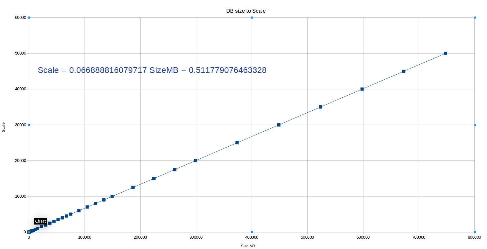
But the thing that has always annoyed me a bit, is the fact that one cannot specify the desired database or table size but has to think in so called "scaling factor" numbers. And we know from documentation, that scaling factor of "1" means 100k rows in the main data table "pgbench_accounts". But how the does scaling factor of 100 (i.e. 10 Million bank accounts) translate to disk size? Which factor do I need to input when wanting to quickly generate a database of 50 GB to see how random updates would perform, in case the dataset does not fit into RAM/shared buffers. Currently there is a bit of trial and error involved 🙁 So how to get rid of the guesswork and be a bit more deterministic? Well I guess one needs a formula that translates input of DB size to scaling factor!

Test data generation

One way to arrive at the magic formula would be to generate a lot of sample data for various scaling factors, measure the resulting on-disk sizes and deriving a formula out of it. That's exactly what I've done.

So I hatched up the script below and booted up a GCE instance, destined to churn the disks nonstop for a bit more than a whole day as it appeared - I'm sorry little computer 🙂 The script is very simple - it runs the pgbench schema initialization with different scaling factors from 1 to 50k and stores the resulting DB/table/index sizes in a table, so that later some statistics/maths could be applied to infer a formula. NB! Postgres version used was 10.1.

psql -c 'create table if not exists init_results (scale int not null, table_size_mb int not null, index_size_mb int not null, db_size_mb int not null);'

SCALES='1 10 50 100 150 200 250 300 350 400 450 500 750 1000 1500 2000 2500 3000 3500 4000 4500 5000 6000 7000 8000 9000 10000 12500 15000 17500 19999 20000 25000 30000 35000 40000 45000 50000'

for x in $SCALES ; do

pgbench -i --unlogged-tables -s $x -n &>/tmp/pgbench.log

SQL=$(cat <<-EOF

insert into init_results select

${x},

(select round(pg_table_size('pgbench_accounts') / 1024^2)),

(select round(pg_relation_size('pgbench_accounts_pkey') / 1024^2)),

(select round(pg_database_size(current_database()) / 1024^2))

EOF

)

echo '$SQL' | psql

done

psql -c 'create table if not exists init_results (scale int not null, table_size_mb int not null, index_size_mb int not null, db_size_mb int not null);'

SCALES='1 10 50 100 150 200 250 300 350 400 450 500 750 1000 1500 2000 2500 3000 3500 4000 4500 5000 6000 7000 8000 9000 10000 12500 15000 17500 19999 20000 25000 30000 35000 40000 45000 50000'

for x in $SCALES ; do

pgbench -i --unlogged-tables -s $x -n &>/tmp/pgbench.log

SQL=$(cat <<-EOF

insert into init_results select

${x},

(select round(pg_table_size('pgbench_accounts') / 1024^2)),

(select round(pg_relation_size('pgbench_accounts_pkey') / 1024^2)),

(select round(pg_database_size(current_database()) / 1024^2))

EOF

)

echo '$SQL' | psql

done

Turning test data into a formula

After the script finished (25h later...note that without the "--unlogged-tables" flag it would take a lot longer), I had a nice table showing how different scaling factors translate to database size on disk, measured in MB (MiB/mebibytes to be exact, i.e. 1MB=1048576 bytes) as this is what the "psql" client is using when reporting object sizes.

So now how to turn this data around so that we get a formula to calculate scaling factors, based on input target DB size? Well I'm sure there are quite some ways and countless Statistics/Data Mining techniques could be applied, but as Data Science is not my strongest skill I thought I'll first take the simplest possible road of using built in statistics functions of a spreadsheet program and see how it fares. If the estimation doesn't look good I could look for something more sophisticated, scikit-learn or such. But luckily it worked out quite well!

Simple regression analysis with LibreOffice

LibreOffice (my office suite of choice) is nowhere near MS Excel but it does have some quite good Statistical Regression functionalities built in and one has options to calculate regression constants together with accuracy coefficients or calculate the formulas and draw them on charts as "Trend Lines". I went the visual way. It goes something like that – create a normal chart, activate it with a double-click and then right click on some data point on the chart and select "Insert Trend Line" from the appearing popup menu. On the next screen one can choose if the "to be fitted" formula for your data should be a simple linear one or a logarithmic/exponential/polynomial. In the case of pgbench data at hand though, after trying out all of them, it appeared that there was no real extra accuracy from the more complex formulas, so I decided to apply KISS here, meaning a simple linear formula. If you look at the script you'll see that we also gathered also size data for the "pgbench_accounts" table and index data, thus for completenes,s I also generated the formulas for calculating scaling factors from target "pgbench_accounts" table/index sizes, but mostly it should not be of interest as the prominent table makes up 99% of the DB size.

The magic formula

So without further ado, below are the resulting formulas and a graph showing how pgbench scale changes according to DB size. I also created a small JSFiddle that you can bookmark here if you happen to work with pgbench a lot.

NB! Accuracy here is not 100% perfect of course as there are some non-linear components (pgbench_accounts.aid changes to int8 from scale 20k, index leaf density varies minimally) but it is really "good enough", meaning <1% accuracy error. Hope you find it useful and would be nice if something similar ends up in "pgbench" tool itself one day.

Target object	Scale Formula
DB	0.0669 * DB_Size_Target_MB - 0.5
Table (pgbench_accounts)	0.0781 * Table_Size_Target_MB
Index (pgbench_accounts_pkey)	0.4668 * Index_Size_Target_MB

Detect PostgreSQL performance problems with ease: Is there a single significantly large and important database in the world which does not suffer from performance problems once in a while? I bet that there are not too many. Therefore, every DBA (database administrator) in charge of PostgreSQL should know how to track down potential performance problems to figure out what is really going on.

Improving PostgreSQL performance beyond parameter tuning

Many people think that changing parameters in postgresql.conf is the real way to success. However, this is not always the case. Sure, more often than not, good database config parameters are highly beneficial. Still, in many cases the real problems will come from some strange query hidden deep in some application logic. It is even quite likely that those queries causing real issues are not the ones you happen to focus on. The natural question now arising is: How can we track down those queries and figure out, what is really going on? My favorite tool to do that is pg_stat_statements, which should always be enabled in my judgement if you are using PostgreSQL 9.2 or higher (please do not use it in older versions).

Enabling pg_stat_statements

To enable pg_stat_statements on your server change the following line in postgresql.conf and restart PostgreSQL:

shared_preload_libraries = 'pg_stat_statements'

Once this module has been loaded into the server, PostgreSQL will automatically start to collect information. The good thing is that the overhead of the module is really really low (the overhead is basically just “noise”).

Then run the following command to create the necessary view to access the data:

CREATE EXTENSION pg_stat_statements;

1	CREATE EXTENSION pg_stat_statements;

The extension will deploy a view called pg_stat_statements and make the data easily accessible.

Detecting slow queries in PostgreSQL

The easiest way to find the most interesting queries is to sort the output of pg_stat_statements by total_time:

SELECT * FROM pg_stat_statements ORDER BY total_time DESC;

1	SELECT * FROM pg_stat_statements ORDER BY total_time DESC;

The beauty here is that the type of query, which is consuming most of time, will naturally show up on top of the listing. The best way is to work your way down from the first to the, say, 10th query and see, what is going on there.
In my judgement there is no way to tune a system without looking at the most time-consuming queries on the database server.

Taking a deep look at PostgreSQL performance problems

pg_stat_statements has a lot more to offer than just the query and the time it has eaten. Here is the structure of the view:

test=# d pg_stat_statements
View 'public.pg_stat_statements'
Column               |     Type         | Collation | Nullable | Default
---------------------+------------------+-----------+----------+---------
 userid              | oid              |           |          |
 dbid                | oid              |           |          |
 queryid             | bigint           |           |          |
 query               | text             |           |          |
 calls               | bigint           |           |          |
 total_time          | double precision |           |          |
 min_time            | double precision |           |          |
 max_time            | double precision |           |          |
 mean_time           | double precision |           |          |
 stddev_time         | double precision |           |          |
 rows                | bigint           |           |          |
 shared_blks_hit     | bigint           |           |          |
 shared_blks_read    | bigint           |           |          |
 shared_blks_dirtied | bigint           |           |          |
 shared_blks_written | bigint           |           |          |
 local_blks_hit      | bigint           |           |          |
 local_blks_read     | bigint           |           |          |
 local_blks_dirtied  | bigint           |           |          |
 local_blks_written  | bigint           |           |          |
 temp_blks_read      | bigint           |           |          |
 temp_blks_written   | bigint           |           |          |
 blk_read_time       | double precision |           |          |
 blk_write_time      | double precision |           |          |

test=# d pg_stat_statements

View 'public.pg_stat_statements'

Column | Type | Collation | Nullable | Default

---------------------+------------------+-----------+----------+---------

userid | oid | | |

dbid | oid | | |

queryid | bigint | | |

query | text | | |

calls | bigint | | |

total_time | double precision | | |

min_time | double precision | | |

max_time | double precision | | |

mean_time | double precision | | |

stddev_time | double precision | | |

rows | bigint | | |

shared_blks_hit | bigint | | |

shared_blks_read | bigint | | |

shared_blks_dirtied | bigint | | |

shared_blks_written | bigint | | |

local_blks_hit | bigint | | |

local_blks_read | bigint | | |

local_blks_dirtied | bigint | | |

local_blks_written | bigint | | |

temp_blks_read | bigint | | |

temp_blks_written | bigint | | |

blk_read_time | double precision | | |

blk_write_time | double precision | | |

It can be quite useful to take a look at the stddev_time column as well. It will tell you if queries of a certain type tend to have similar runtimes or not. If the standard deviation is high you can expect some of those queries to be fast and some of them to be slow, which might lead to bad user experience.

The “rows” column can also be quite informative. Suppose 1000 calls have returned 1.000.000.000 rows: It actually means that every call has returned 1 million rows in average. It is easy to see that returning so much data all the time is not a good thing to do.

If you want to check if a certain type of query shows bad caching performance, the shared_* will be of interest. In short: PostgreSQL is able to tell you the cache hit rate of every single type of query in case pg_stat_statements has been enabled.

It also makes sense to take a look at the temp_blks_* fields. Whenever PostgreSQL has to go to disk to sort or to materialize, temporary blocks will be needed.

Finally there are blk_read_time and blk_write_time. Usually those fields are empty unless track_io_timing is turned on. The idea here is to be able to measure the amount of time a certain type of query spends on I/O. It will allow you to answer the question whether your system is I/O bound or CPU bound. In most cases it is a good idea to turn on I/O timing because it will give you vital information.

Dealing with Java and Hibernate

pg_stat_statements delivers good information. However, in some cases it can cut off the query because of a config variable:

test=# SHOW track_activity_query_size;
track_activity_query_size
---------------------------
1024
(1 row)

test=# SHOW track_activity_query_size;

track_activity_query_size

---------------------------

1024

(1 row)

For most applications 1024 bytes are absolutely enough. However, this is usually not the case if you are running Hibernate or Java. Hibernate tends to send insanely long queries to the database and thus the SQL code might be cut off long before the relevant parts start (e.g. the FROM-clause etc.). Therefore it makes a lot of sense to increase track_activity_query_size to a higher value (maybe 32.786).

Helpful queries to detect bottlenecks in PostgreSQL

There is one query I have found especially useful in this context: The following query shows 20 statements, which need a lot of time:

test=# SELECT substring(query, 1, 50) AS short_query,
              round(total_time::numeric, 2) AS total_time,
              calls,
              round(mean_time::numeric, 2) AS mean,
              round((100 * total_time / sum(total_time::numeric) OVER ())::numeric, 2) AS percentage_cpu
FROM  pg_stat_statements
ORDER BY total_time DESC
LIMIT 20;
           short_query                              | total_time | calls | mean | percentage_cpu
----------------------------------------------------+------------+-------+------+----------------
SELECT name FROM (SELECT pg_catalog.lower(name) A   | 11.85      | 7     | 1.69 | 38.63
DROP SCHEMA IF EXISTS performance_check CASCADE;    | 4.49       | 4     | 1.12 | 14.64
CREATE OR REPLACE FUNCTION performance_check.pg_st  | 2.23       | 4     | 0.56 | 7.27
SELECT pg_catalog.quote_ident(c.relname) FROM pg_c  | 1.78       | 2     | 0.89 | 5.81
SELECT a.attname, +                                 | 1.28       | 1     | 1.28 | 4.18
SELECT substring(query, ?, ?) AS short_query,roun   | 1.18       | 3     | 0.39 | 3.86
CREATE OR REPLACE FUNCTION performance_check.pg_st  | 1.17       | 4     | 0.29 | 3.81
SELECT query FROM pg_stat_activity LIMIT ?;         | 1.17       | 2     | 0.59 | 3.82
CREATE SCHEMA performance_check;                    | 1.01       | 4     | 0.25 | 3.30
SELECT pg_catalog.quote_ident(c.relname) FROM pg_c  | 0.92       | 2     | 0.46 | 3.00
SELECT query FROM performance_check.pg_stat_activi  | 0.74       | 1     | 0.74 | 2.43
SELECT * FROM pg_stat_statements ORDER BY total_ti  | 0.56       | 1     | 0.56 | 1.82
SELECT query FROM pg_stat_statements LIMIT ?;       | 0.45       | 4     | 0.11 | 1.45
GRANT EXECUTE ON FUNCTION performance_check.pg_sta  | 0.35       | 4     | 0.09 | 1.13
SELECT query FROM performance_check.pg_stat_statem  | 0.30       | 1     | 0.30 | 0.96
SELECT query FROM performance_check.pg_stat_activi  | 0.22       | 1     | 0.22 | 0.72
GRANT ALL ON SCHEMA performance_check TO schoenig_  | 0.20       | 3     | 0.07 | 0.66
SELECT query FROM performance_check.pg_stat_statem  | 0.20       | 1     | 0.20 | 0.67
GRANT EXECUTE ON FUNCTION performance_check.pg_sta  | 0.19       | 4     | 0.05 | 0.62
SELECT query FROM performance_check.pg_stat_statem  | 0.17       | 1     | 0.17 | 0.56
(20 rows)

test=# SELECT substring(query, 1, 50) AS short_query,

round(total_time::numeric, 2) AS total_time,

calls,

round(mean_time::numeric, 2) AS mean,

round((100 * total_time / sum(total_time::numeric) OVER ())::numeric, 2) AS percentage_cpu

FROM pg_stat_statements

ORDER BY total_time DESC

LIMIT 20;

short_query | total_time | calls | mean | percentage_cpu

----------------------------------------------------+------------+-------+------+----------------

SELECT name FROM (SELECT pg_catalog.lower(name) A | 11.85 | 7 | 1.69 | 38.63

DROP SCHEMA IF EXISTS performance_check CASCADE; | 4.49 | 4 | 1.12 | 14.64

CREATE OR REPLACE FUNCTION performance_check.pg_st | 2.23 | 4 | 0.56 | 7.27

SELECT pg_catalog.quote_ident(c.relname) FROM pg_c | 1.78 | 2 | 0.89 | 5.81

SELECT a.attname, + | 1.28 | 1 | 1.28 | 4.18

SELECT substring(query, ?, ?) AS short_query,roun | 1.18 | 3 | 0.39 | 3.86

CREATE OR REPLACE FUNCTION performance_check.pg_st | 1.17 | 4 | 0.29 | 3.81

SELECT query FROM pg_stat_activity LIMIT ?; | 1.17 | 2 | 0.59 | 3.82

CREATE SCHEMA performance_check; | 1.01 | 4 | 0.25 | 3.30

SELECT pg_catalog.quote_ident(c.relname) FROM pg_c | 0.92 | 2 | 0.46 | 3.00

SELECT query FROM performance_check.pg_stat_activi | 0.74 | 1 | 0.74 | 2.43

SELECT * FROM pg_stat_statements ORDER BY total_ti | 0.56 | 1 | 0.56 | 1.82

SELECT query FROM pg_stat_statements LIMIT ?; | 0.45 | 4 | 0.11 | 1.45

GRANT EXECUTE ON FUNCTION performance_check.pg_sta | 0.35 | 4 | 0.09 | 1.13

SELECT query FROM performance_check.pg_stat_statem | 0.30 | 1 | 0.30 | 0.96

SELECT query FROM performance_check.pg_stat_activi | 0.22 | 1 | 0.22 | 0.72

GRANT ALL ON SCHEMA performance_check TO schoenig_ | 0.20 | 3 | 0.07 | 0.66

SELECT query FROM performance_check.pg_stat_statem | 0.20 | 1 | 0.20 | 0.67

GRANT EXECUTE ON FUNCTION performance_check.pg_sta | 0.19 | 4 | 0.05 | 0.62

SELECT query FROM performance_check.pg_stat_statem | 0.17 | 1 | 0.17 | 0.56

(20 rows)

The last column is especially noteworthy: It tells us the percentage of total time burned by a single query. It will help you to figure out whether a single statement is relevant to overall performance problems or not.

Many people ask about index scans in PostgreSQL. This blog is meant to be a basic introduction to the topic. Many people aren't aware of what the optimizer does when a single query is processed. I decided to show how a table can be accessed and give examples. Let's get started with PostgreSQL indexing.

Indexes are the backbone of good performance. Without proper indexing, your PostgreSQL database might be in dire straits and end users might complain about slow queries and bad response times. It therefore makes sense to see which choices PostgreSQL makes when a single column is queried.

Preparing some demo data in PostgreSQL

To show you how things work we can use a table:

test=# CREATE TABLE sampletable (x numeric);
CREATE TABLE

1 2	test=# CREATE TABLE sampletable (x numeric); CREATE TABLE

If your table is almost empty, you will never see an index scan, because it might be too much overhead to consult an index - it is cheaper to just scan the table directly and throw away whatever rows which don't match your query.

So to demonstrate how an index actually works, we can add 10 million random rows to the table we just created before:

test=# INSERT INTO sampletable
         SELECT random() * 10000
         FROM generate_series(1, 10000000);
INSERT 0 10000000

test=# INSERT INTO sampletable

SELECT random() * 10000

FROM generate_series(1, 10000000);

INSERT 0 10000000

Then an index is created:

test=# CREATE INDEX idx_x ON sampletable(x);
CREATE INDEX

1 2	test=# CREATE INDEX idx_x ON sampletable(x); CREATE INDEX

After loading so much data, it is a good idea to create optimizer statistics in case autovacuum has not caught up yet. The PostgreSQL optimizer needs these statistics to decide on whether to use an index or not:

test=# ANALYZE ; 
ANALYZE

1 2	test=# ANALYZE ; ANALYZE

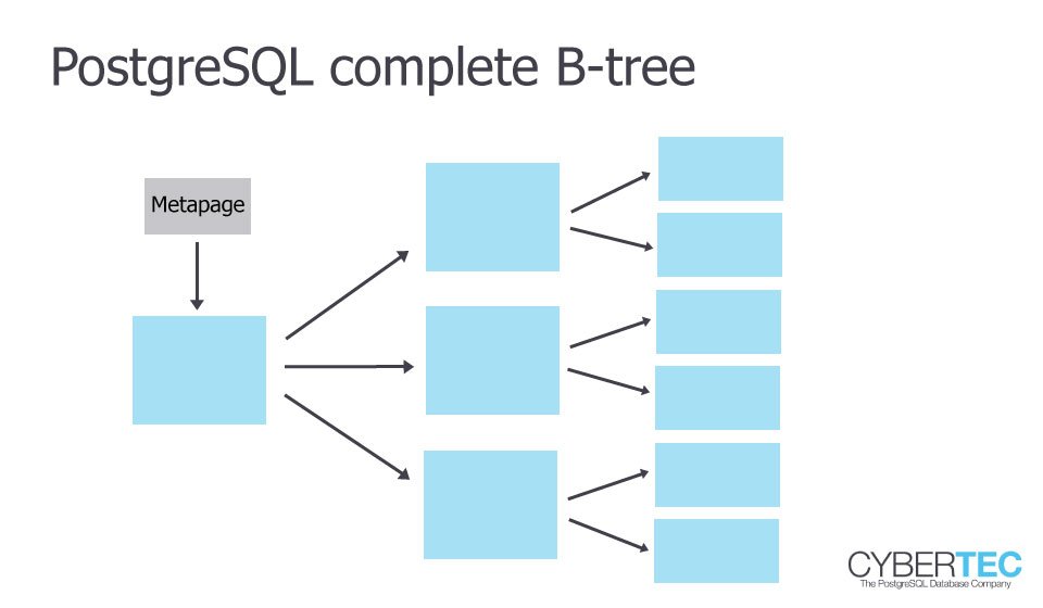
In PostgreSQL a btree uses Lehman-Yao High-Concurrency btrees (which will be covered in more detail in a later blog).

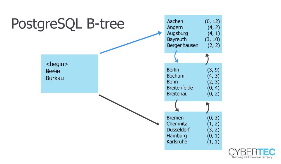
Selecting a small subset of data in PostgreSQL

When only a small set of rows is selected, PostgreSQL can directly ask the index. In this case it can even use an “Index Only Scan” because all columns needed are actually already in the index:

test=# explain SELECT * FROM sampletable WHERE x = 42353;
                               QUERY PLAN
-----------------------------------------------------------------------
Index Only Scan using idx_x on sampletable (cost=0.43..8.45 rows=1 width=11)
      Index Cond: (x = '42353'::numeric)
(2 rows)

test=# explain SELECT * FROM sampletable WHERE x = 42353;

QUERY PLAN

-----------------------------------------------------------------------

Index Only Scan using idx_x on sampletable (cost=0.43..8.45 rows=1 width=11)

Index Cond: (x = '42353'::numeric)

(2 rows)

Selecting only a handful of rows will be super efficient using the index. However, if more data is selected, scanning the index AND the table will be too expensive.

PostgreSQL indexing: Selecting a lot of data from a table in PostgreSQL

However, if you select a LOT of data from a table, PostgreSQL will fall back to a sequential scan. In this case, reading the entire table and just filtering out a couple of rows is the best way to do things.

Here is how it works:

test=# explain SELECT * FROM sampletable WHERE x < 42353;
                            QUERY PLAN
---------------------------------------------------------------
Seq Scan on sampletable (cost=0.00..179054.03 rows=9999922 width=11)
    Filter: (x < '42353'::numeric)
(2 rows)

test=# explain SELECT * FROM sampletable WHERE x < 42353;

QUERY PLAN

---------------------------------------------------------------

Seq Scan on sampletable (cost=0.00..179054.03 rows=9999922 width=11)

Filter: (x < '42353'::numeric)

(2 rows)

PostgreSQL will filter out those unnecessary rows and just return the rest. This is really the ideal thing to do in this case. A sequential scan is therefore not always bad - there are use cases where a sequential scan is actually perfect.

Still: Keep in mind that scanning large tables sequentially too often will take its toll at some point.

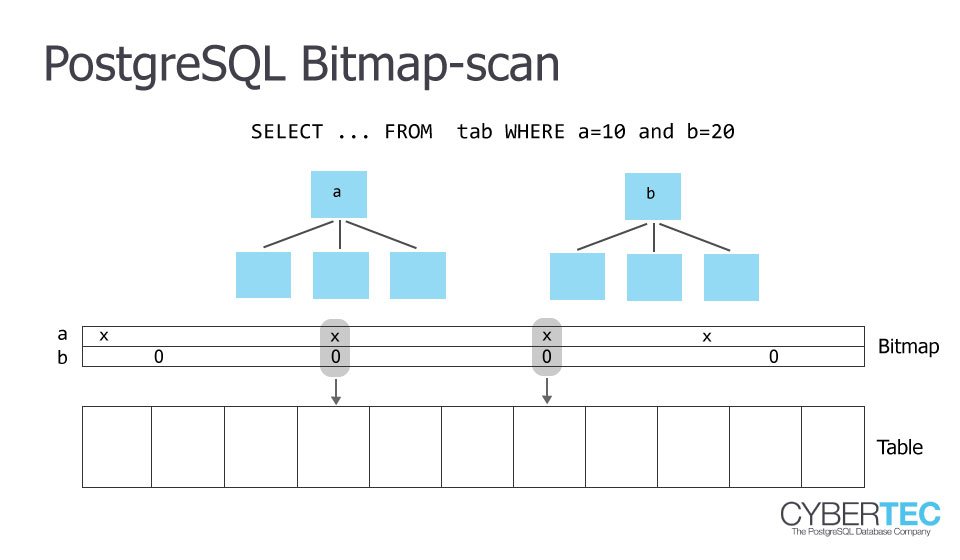
PostgreSQL: Making use of bitmap scans

If you only select a handful of rows, PostgreSQL will decide on an index scan - if you select a majority of the rows, PostgreSQL will decide to read the table completely. But what if you read too much for an index scan to be efficient but too little for a sequential scan? The solution to the problem is to use a bitmap scan. The idea behind a bitmap scan is that a single block is only used once during a scan. It can also be very helpful if you want to use more than one index to scan a single table.

Here is what happens:

test=# explain SELECT * FROM sampletable WHERE x < 423;
                                    QUERY PLAN
----------------------------------------------------------------------------
Bitmap Heap Scan on sampletable (cost=9313.62..68396.35 rows=402218 width=11)
       Recheck Cond: (x < '423'::numeric)
       -> Bitmap Index Scan on idx_x (cost=0.00..9213.07 rows=402218 width=0)
          Index Cond: (x < '423'::numeric)
(4 rows)

test=# explain SELECT * FROM sampletable WHERE x < 423;

QUERY PLAN

----------------------------------------------------------------------------

Bitmap Heap Scan on sampletable (cost=9313.62..68396.35 rows=402218 width=11)

Recheck Cond: (x < '423'::numeric)

-> Bitmap Index Scan on idx_x (cost=0.00..9213.07 rows=402218 width=0)

Index Cond: (x < '423'::numeric)

(4 rows)

PostgreSQL will first scan the index and compile those rows / blocks which are needed at the end of the scan. Then PostgreSQL will take this list and go to the table to really fetch those rows. The beauty is that this mechanism even works if you are using more than just one index.

Bitmaps scans are therefore a wonderful contribution to performance.

Read more about how foreign key indexing affects performance, and how to find missing indexes in Laurenz Albe's blog.

In order to receive regular updates on important changes in PostgreSQL, subscribe to our newsletter, or follow us on Twitter, Facebook, or LinkedIn.

By Kaarel Moppel - The last couple of weeks, I've had the chance to work on our Open Source PostgreSQL monitoring tool called pgwatch2 and implemented some stuff that was in the queue. Changes include only a couple of fixes and a lot of new features... so hell, I'm calling it "Feature Pack 3"... as we've had some bigger additions in the past. Read on for a more detailed overview on the most important new stuff.

Becoming "Enterprizy"

The focus word this time could be "Enterprise". Meaning - firstly trying to make pgwatch2 easier to deploy for larger companies, who maybe need to think about security or container orchestration and secondly also adding robustness. Security even got some special attention – now there's a pgwatch2 version suitable for running on OpenShift, i.e. Docker process runs under an unprivileged user. But there are also quite some new dashboards (see screenshots at the end), like the long-awaited "Top N queries", that should delight all "standard" users and also some other smaller UI improvements.

And please do let us know on GitHub if you’re still missing something in the tool or are having difficulties with something – I myself think I've lost the ability to look at the tool with beginner eyes. Thus - any feedback would be highly appreciated!

Project GitHub link – here.

Version 1.3 full changelog – here.

Most important changes for v1.3.0

"Non-root" Docker support

Suitable for example for OpenShift deployments.

Explicit Docker volumes added to Postgres, Grafana, InfluxDB and pgwatch2 config

Using volumes was of course also possible before, but people didn't seem to think about it, so now it's more explicit. Volumes helps a lot for long term Docker deployments as it makes updating to new image versions quite easy compared to dump/restore.

Docker files for deploying "non-root" components separately

These can be used to do some advanced orchestrated setups. See the "docker" folder for details. There are also latest images available on Docker Hub, but it's meant more for DIY still.

Better Grafana access control vie env. variables

Now it is possible to turn off anonymous access and set admin user/password.

New "AWS CloudWatch overview" dashboard

One can now easily monitor/alert on a mix of on-prem and AWS RDS managed DBs.

New dashboard for PgBouncer statistics

Visualizes PgBouncer "SHOW STATS" commands. NB! Requires config DB schema
change for existing setups as a new "datasource type" field was introduced.

New dashboard for "Top N" time consuming/frequent/slowest/IO-hungry queries added

Now one can see based on pg_stat_statements info, exactly which queries are the costliest (4 criteria available) over a user selected timeperiod. Lots of people have asked for that, so please, enjoy!

New dashboard - "Biggest relations treemap"

Helps to visually highlight biggest tables/indexes. Uses a custom plugin for Grafana.

InfluxDB HA support added, i.e. writing metrics to 2 independent DBs

Metrics gathering daemon can now store all gathered metrics in 2 independent InfluxDBs...so kind of homebrewn clustering. For real clustering one needs the commercial Influx version so be sure to check it out also if needing extra robustness, seems like a great product.

Gatherer daemon robustness - a ringbuffer of max 100k metrics datapoints introduced

Previously if Influx was down metrics were gathered and saved in daemon memory till things blew up. 100k datasets translates into ~ 2GB of RAM.

InfluxDB metrics retention period now configurable via ENV

Variable is called PW2_IRETENTIONDAYS. Default is 90 days.

"Change detection" doesn't expect superuser rights on the monitored DB anymore

Web UI security - respecting the "only SSL connections" ENV variable also for Postgres

Web UI security - now possible to disable exposing of component logs

README improvements - a new section on custom deployments

README improvements - a new docu on all available ENV variables, per subcomponent

pgwatch2 is constantly being improved and new features are added. Learn more >>

Screenshots of new Dashboards

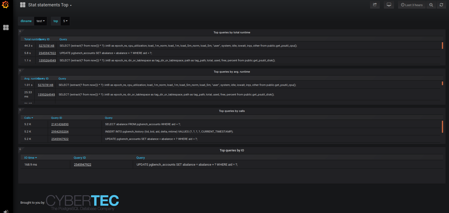
Stat Statements Top

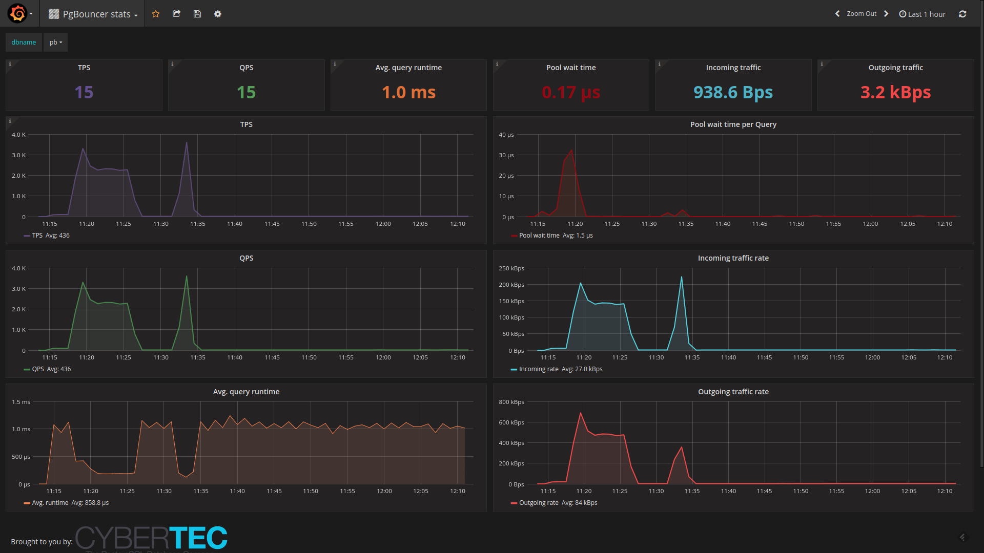
PgBouncer Stats

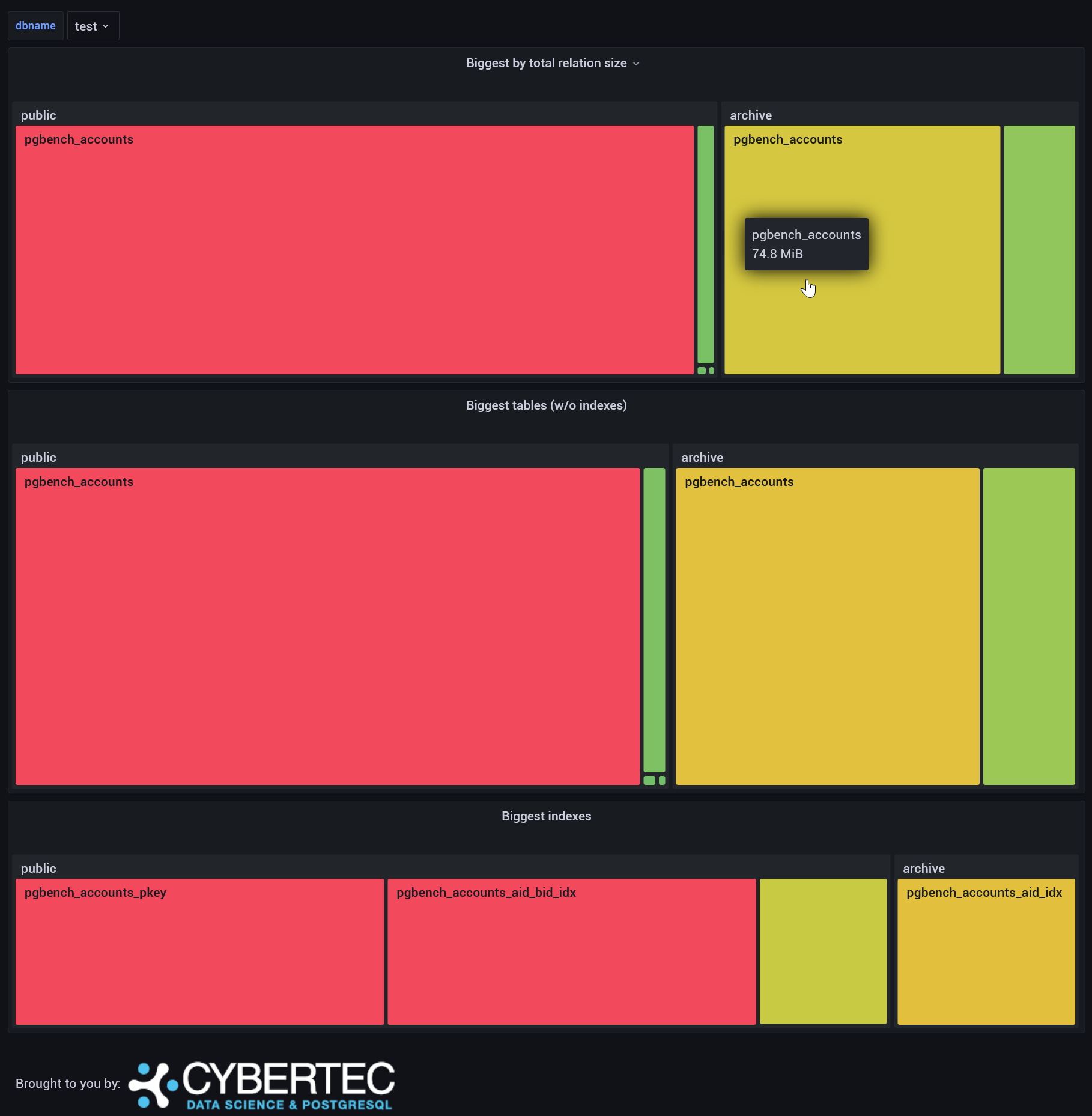
Biggest relations

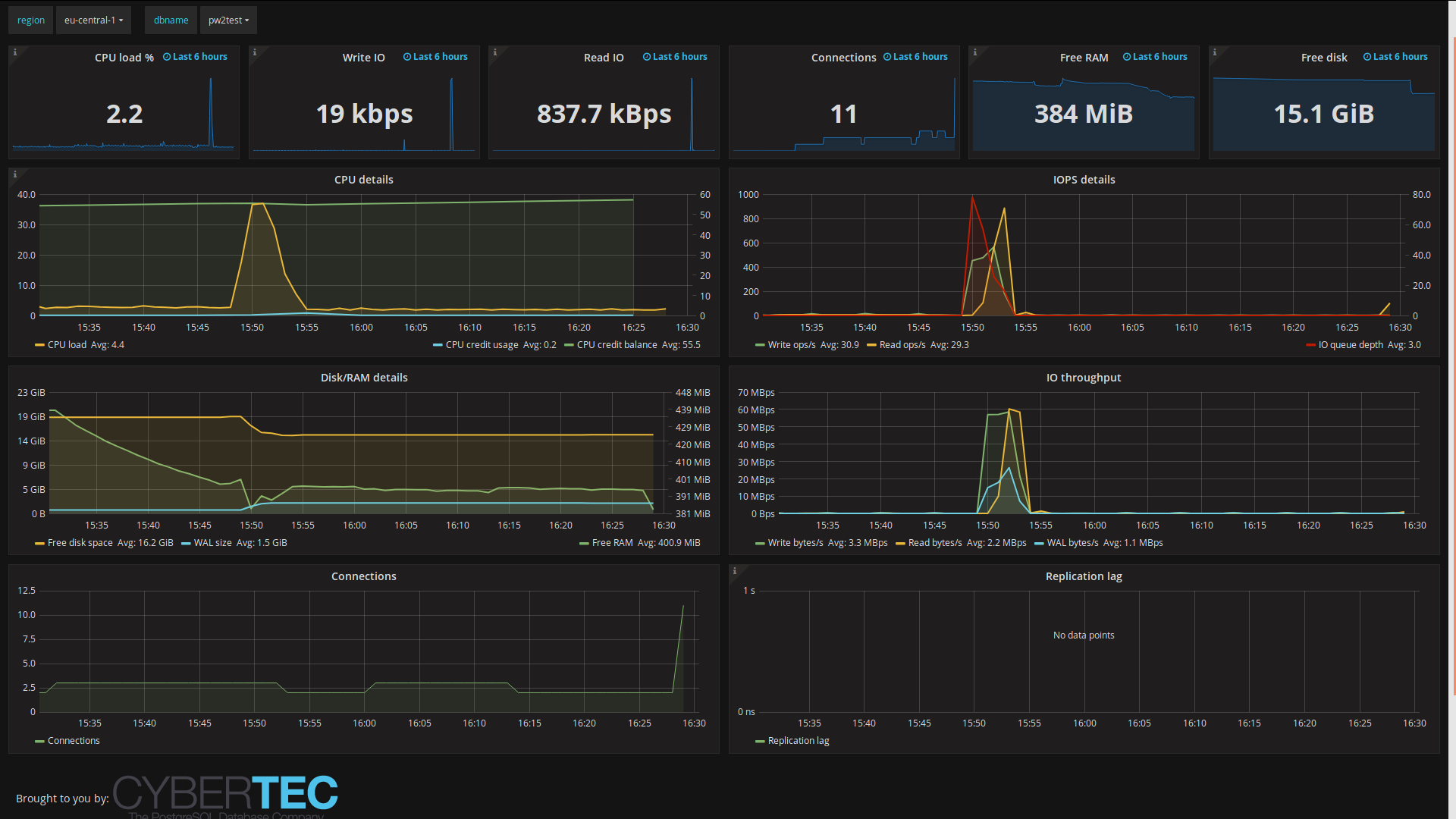
AWS RDS overview

About sequences

New developments in PostgreSQL v10

Identity columns

New system catalog pg_sequence

Transactional DDL for sequences

Performance regression with ALTER SEQUENCE

PostgreSQL and the optimizer: What they do to views

Inlining and flattening

Joining views

Destructive behavior

Conclusion

Test data generation

Turning test data into a formula

Simple regression analysis with LibreOffice

The magic formula

Improving PostgreSQL performance beyond parameter tuning

Enabling pg_stat_statements

Detecting slow queries in PostgreSQL

Taking a deep look at PostgreSQL performance problems

Dealing with Java and Hibernate

Helpful queries to detect bottlenecks in PostgreSQL

Preparing some demo data in PostgreSQL

Selecting a small subset of data in PostgreSQL

PostgreSQL indexing: Selecting a lot of data from a table in PostgreSQL

PostgreSQL: Making use of bitmap scans

Becoming "Enterprizy"

Most important changes for v1.3.0

Screenshots of new Dashboards

New system catalog `pg_sequence`

Performance regression with `ALTER SEQUENCE`