In SQL the GROUP BY clause groups records into summary rows and turns large amounts of data into a smaller set. GROUP BY returns one records for each group. While most people know how to use GROUP BY not many actually know how to squeeze the last couple of percentage points out of the query. There is a small optimization, which can help you to speed up things by a couple of percents quite reliably. If you want to speed up GROUP BY clauses, this post is for you.

Creating a test data set in PostgreSQL

To prepare ourselves for the aggregation we first have to generate some data:

The interesting part is that the first column only has 2 distinct values while the second column will contain 10.000 different values. That is going to be of great importance for our optimization efforts.

Let us VACUUM the table to set hint bits and to build optimizer statistics. To make those execution plans more readable I also decided to turn off parallel queries:

Running an aggregation

Now that the is in place the first tests can be started:

PostgreSQL will read the entire table sequentially and perform a hash aggregate. As you can see most of the time is burned by the hash aggregate (3.3 seconds minus 636 milliseconds). The resultset contains 6000 rows. However, we can do better. Keep in mind that the first column does not contain as many different values as the second column. That will have some implications as far as the hash aggregate is concerned. Let us try to play around with the GROUP BY clause

Changing aggregation order can improve performance

Let us run the same query again. But this time we won’t use “GROUP BY x, y” but instead use “GROUP BY y, x”. The result of the statement will be exactly the same as before (= 10.000 groups). However, the slightly modified query will be faster:

Wow, the query has improved considerably. We saved around 400ms, which is a really big deal. The beauty is that we did not have to rearrange the data, change the table structure, adjust memory parameters or make any other changes to the server. All I did was to change the order in which PostgreSQL aggregated the data.

Conclusions...

Which conclusions can developers draw from this example? If you are grouping by many different columns: Take the ones containing more distinct values first and group by the less frequent values later. It will make the hash aggregate run more efficiently in many cases. Also try to make sure that work_mem is high enough to make PostgreSQL trigger a hash aggregate in the first place. Using a hash is usually faster than letting PostgreSQL use the “group aggregate”.

It is very likely that future versions of PostgreSQL (maybe starting with PostgreSQL 12?) will already do this kind of change automatically. A patch has already been proposed by Teodor Sigaev and I am quite confident that this kind of optimization will make it into PostgreSQL 12. However, in the meantime it should be easy to make the change by hand and enjoy a nice, basically free speedup.

If you want to learn more about GROUP BY, aggregations and work_mem in general, consider checking out my blog post about this topic. On behalf of the entire team I wish everybody “happy performance tuning”. If you want to learn more about aggregation and check out Teodor Sigaev's patch, check out the PostgreSQL mailing list.

If you want to learn more about performance tuning, advanced SQL and so on, consider checking out one of our posts about window functions and analytics.

 

---

In order to receive regular updates on important changes in PostgreSQL, subscribe to our newsletter, or follow us on Facebook or LinkedIn.

Foreign data wrappers are one of the most widely used feature in PostgreSQL. People simply like foreign data wrappers and we can expect that the community will add even more features as we speak. As far as the postgres_fdw is concerned there are some hidden tuning options which are not widely known by users. So let's see how we can speed up the PostgreSQL foreign data wrapper.

Foreign data wrappers: Creating a “database link”

To show how things can be improved we first have to create some sample data in “adb”, which can then be integrated into some other database:

In this case I have simply loaded 100.000 rows into a very simple table. Let us now create the foreign data wrapper (or “database link” as Oracle people would call it). The first thing to do is to enable the postgres_fdw extension in “bdb”.

In the next step we have to create the “SERVER”, which points to the database containing our sample table. CREATE SERVER works like this:

Once the foreign server is created the users we need can be mapped:

In this example the user mapping is really easy. We simply want the current user to connect to the remote database as “hs” (which happens to be my superuser).

Finally, we can link the tables. The easiest way to do that is to use “IMPORT FOREIGN SCHEMA”, which simply fetches the remote data structure and turns everything into a foreign table.

The command is really easy and shown in the next listing:

As you can see PostgreSQL has nicely created the schema for us and we are basically ready to go.

Testing postgres_fdw performance

When we query our 100.000 row table we can see that the operation can be done in roughly 7.5 milliseconds:

Let us connect to “bdb” now and see, how long the other database needs to read the data:

In this example you can see that 90 milliseconds are burned to do the same thing. So why is that? Behind the scenes the foreign data wrapper creates a cursor and fetches data in really small chunks. By default, only 50 rows are fetched at a time. This translates to thousands of network requests. If our two database servers would be further away, things would take even longer – A LOT longer. Network latency plays a crucial role here and performance can really suffer.

One way to tackle the problem is to fetch larger chunks of data at once to reduce the impact of the network itself. ALTER SERVER will allow us to set the “fetch_size” to a large enough value to reduce network issues without increasing memory consumption too much. Here is how it works:

Let us run the test and see, what will happen:

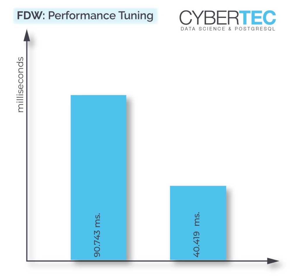
Wow, we have managed to more than double the speed of the query. Of course, the foreign data wrapper is still slower than a simple local query. However, the speedup is considerable and it definitely makes sense to toy around with the parameters to tune it.

If you want to learn more about Foreign Data Wrappers, performance and monitoring, check out one of our other blog posts.

 

---

In order to receive regular updates on important changes in PostgreSQL, subscribe to our newsletter, or follow us on Facebook or LinkedIn.

Database people dealing with natural languages are all painfully aware of the fact that encodings, special characters, accents and alike are usually hard to deal with. This is especially true if you want to implement search in a user-friendly way. This post describes the PG extension unaccent.

Consider the following example in PostgreSQL: My name contains a couple of super inconvenient special characters, which will cause issues for people around the globe. The correct spelling of my surname is “Schönig”, which is pretty hard to type on most keyboards I have seen around the world. And: Who cares about my special characters anyway? People might just want to type in “Schonig” into some search form and find information about me (ideally related to PostgreSQL and database work).

Here is the problem:

The “=” operator compares those two strings and concludes that those two strings are not identical. Therefore, the correct answer is “false”. While that is true from a technical point of view it might be a real issue and end users might be unsatisfied with the result. Problems like that can make daily life pretty hard. A solution to the problem is therefore needed.

PostgreSQL provides a useful extension

If you want to improve your user experience you can turn to the “unaccent” extension, which is shipped as part of the PostgreSQL contrib package. Installing it is really easy:

In the next step you can call the “unaccent” function to clean a string and turn it into something more useful. This is what happens when we use this function on my name and the name of my PostgreSQL support company:

The beauty is that we can easily compare strings in a more tolerant and more user-friendly way:

In both cases, PostgreSQL will return true, which is exactly what we want.

Indexing

When using unaccent there is one thing, which you should keep in mind. Here is an example:

PostgreSQL supports the creation of indexes on functions. However, a functional index has to return an immutable result, which is not the case here. If you want to index on an unaccented string you have to create an additional column, which contains a pre-calculated value (“materialized”). Otherwise, it's just not possible.

 

---

In order to receive regular updates on important changes in PostgreSQL, subscribe to our newsletter, or follow us on Facebook or LinkedIn.

 

Many people know that explicit table locks with LOCK TABLE are bad style and usually a consequence of bad design. The main reason is that they hamper concurrency and hence performance.

Through a recent support case I learned that there are even worse effects of explicit table locks.

Table locks

Before an SQL statement uses a table, it takes the appropriate table lock. This prevents concurrent use that would conflict with its operation. For example, reading from a table will take a ACCESS SHARE lock which will conflict with the ACCESS EXCLUSIVE lock that TRUNCATE needs.

You can find a description of the individual lock levels in the documentation. There is also the matrix that shows which lock levels conflict with each other.

You don't have to perform these table locks explicitly, PostgreSQL does it for you automatically.

Explicit table locks with the LOCK TABLE statement

You can also explicitly request locks on a table with the LOCK statement:

LOCK [ TABLE ] [ ONLY ] name [ * ] [, ...] [ IN lockmode MODE ] [ NOWAIT ]

There are some cases where it is useful and indicated to use such an explicit table lock. One example is a bulk update of a table, where you want to avoid deadlocks with other transactions that modify the table at the same time. In that case you would use a SHARE lock on the table that prevents concurrent data modifications:

Typical mistakes with LOCK TABLE

Unfortunately, most people don't think hard enough and just use “LOCK atable” without thinking that the default lock mode is ACCESS EXCLUSIVE, which blocks all concurrent access to the table, even read access. This harms performance more than necessary.

But most of the time, tables are locked because developers don't know that there are less restrictive ways to achieve what they want:

• You don't want concurrent transactions to modify a row between the time you read it and the time you update it? Use SELECT ... FOR UPDATE!
  If concurrent modifications are unlikely and you are not sure that you are actually going to modify the row, a REPEATABLE READ transaction may be even better. That means that you have to be ready to retry the operation if the UPDATE fails due to a serialization error.
• You want to perform several SELECTs on the table and want to be sure that nobody modifies the table between your statements? Use a transaction with REPEATABLE READ isolation level, so that you see a consistent snapshot of the database!
• You want to get a row from a table, process it and then remove it? Use DELETE ... RETURNING, then the row will be locked immediately!
• You want to implement a queue where workers should grab different items and process them? Use SELECT ... LIMIT 1 FOR UPDATE SKIP LOCKED!
• You want to synchronize concurrent processes with database techniques? Use advisory locks!

LOCK TABLE versus autovacuum

It is necessary that autovacuum processes a table from time to time so that

• dead tuples are removed so that the space can be reused
• the free space map and the visibility map of the table are maintained
• table rows get “frozen” (marked as unconditionally all-visible) before the transaction counter wraps around

Now VACUUM requires a SHARE UPDATE EXCLUSIVE lock on the table. This conflicts with the lock levels people typically use to explicitly lock tables, namely SHARED and ACCESS EXCLUSIVE. (As I said, the latter lock is usually used by mistake.)

Now autovacuum is designed to be non-intrusive. If any transaction that that wants to lock a table is blocked by autovacuum, the deadlock detector will cancel the autovacuum process after a second of waiting. You will see this message in the database log:

The autovacuum launcher process will soon start another autovacuum worker for this table, so this is normally no big problem. Note that “normal” table modifications like INSERT, UPDATE and DELETE do not require locks that conflict with VACUUM!

How things can go wrong

If you use LOCK on a table frequently, there is a good chance that autovacuum will never be able to successfully process that table. This is because it is designed to run slowly, again in an attempt not to be intrusive.

Then dead tuples won't get removed, live tuples won't get frozen, and the table will grow (“get bloated” in PostgreSQL jargon). The bigger the table grows, the less likely it becomes that autoacuum can finish processing it. This can go undetected for a long time unless you monitor the number of dead tuples for each table.

The ugly end

Eventually, though, the sticky brown substance is going to hit the ventilation device. This will happen when there are non-frozen live rows in the table that are older than autovacuum_freeze_max_age. Then PostgreSQL knows that something has to be done to prevent data corruption due to transaction counter wrap-around. It will start autovacuum in “anti-wraparound mode” (you can see that in pg_stat_activity in recent PostgreSQL versions).

Such an anti-wraparound autovacuum will not back down if it blocks other processes. The next LOCK statement will block until autovacuum is done, and if it is an ACCESS EXCLUSIVElock, all other transactions will queue behind it. Processing will come to a sudden stop. Since by now the table is probably bloated out of proportion and autovacuum is slow, this will take a long time.

If you cancel the autovacuum process or restart the database, the autovacuum will just start running again. Even if you disable autovacuum (which is a really bad idea), PostgreSQL will launch the anti-wraparound autovacuum. The only way to resume operation for a while is to increase autovacuum_freeze_max_age, but that will only make things worse eventually: 1 million transactions before the point at which you would suffer data corruption from transaction counter wrap-around, PostgreSQL will shut down and can only be started in single-user mode for a manual VACUUM.

How can I avoid this problem?

First, if you already have the problem, declare downtime, launch an explicit VACUUM (FULL, FREEZE) on the table and wait until it is done.

To avoid the problem:

• Don't use LOCK on a routine basis. Once a day for the nightly bulk load is fine, as long as autovacuum has enough time to finish during the day.
• Tune autovacuum to run more aggressively and hence faster. This can be done by increasing autovacuum_vacuum_cost_limit and reducing autovacuum_vacuum_cost_delay.
• Use PostgreSQL 9.6 or later. Anti-wraparound autovacuum has been improved in 9.6; it now skips pages with only frozen rows to speed up processing.

 

---

In order to receive regular updates on important changes in PostgreSQL, subscribe to our newsletter, or follow us on Twitter, Facebook, or LinkedIn.

Pavel Stehule recently wrote the post "Don't use SQL keywords as PLpgSQL variable names" describing the situation when internal stored routine variable names match PostgreSQL keywords.

But the problem is not only in keywords but also for plpgsql variable names. Consider:

Output:

OK, at least we have no hidden error like in Pavel's case. Let's try to fix it specifying an alias for the table name:

Output:

Seems better, but still parser cannot distinguish the variable name from column name. Of course, we may use variable placeholders instead of names. So, the quick dirty fix is like:

In addition, pay attention that human variable doesn't produce an error, even though it shares the same name with the target table. I personally do not like using $1 placeholders in code, so my suggestion would be (of course, if you don't want to change parameter name):

The same rules apply to plpgsql procedures.

To find out more about plpgsql procedures, see this blog post.