By Kaarel Moppel - If you read this blog post the new PostgreSQL version will be probably already officially released to the public for wider usage...but seems some eager DBA already installed the last week’s Release Candidate 1 and took it for a spin 😉 The “spin” though takes 3 days to run for my scripts, so that’s the reason I didn’t want to wait for the official release.
As this is an RC, and some things could change, etc, just a very brief posting this time with some synthetic pgbench test numbers that I got from my testing laid out for you and a mini conclusion in the end.
The source code statistics, by the way, again look very similar to last year's v12 release, with some very slight decrease in the number of changes done (which on the other hand could be just chunked into larger pieces) so one might assume that overall we would get a very stable release.
|
1 2 3 4 5 |
git diff --shortstat REL_12_4..REL_13_RC1 3109 files changed, 257376 insertions(+), 198880 deletions(-) git log --oneline REL_12_4..REL_13_RC1 | wc -l 2216 |
Test hardware was my good old testing workstation: 4 CPU, 16GB RAM, SATA SSD
OS: A clean install of Ubuntu Server 18.04.5 LTS (Bionic Beaver),
Postgres: v12.4 and v13rc1 self-compiled, all default postgresql.conf parameters except a few “standard” tunings:
|
1 2 3 4 5 |
shared_buffers=4GB logging_collector=on shared_preload_libraries=’pg_stat_statements’ checkpoint_completion_target=0.9 synchronous_commit=off |
Note though that the last parameter “synchronous_commit” is not really a standard setting...but disabling it for testing generally makes sense as we’re not really interested in testing the IO syncing capabilities, but we rather want to move forward with our transactions to push through more “transactions per second” to possibly spot some algorithmic differences. Also, note that pgbench “scaling factor” was selected in a way that the generated dataset would fit mostly into memory for the same purpose.
All timings measured via ‘pg_stat_statements’, which should give the most accurate information.
1 transaction = 5 operations: 3x UPDATE, 1x INSERT, 1x SELECT, 4h runtime per PG version / scale pair, 2 concurrent clients.
TPS improvement for scale 200 (Shared buffers): 4662 vs 4660 ~ 0%
TPS improvement for scale 1200: 249.6 vs 247.9 ~ -0.7%
Timing info for the most costly operation: UPDATE pgbench_accounts SET abalance = abalance + $1 WHERE aid = $2
| Scale | Mean time (ms) | Change % | Stddev (ms) | Change % | |
| 12.4 | 200 (Shared Buffers) | 0.0291 | 3.47 | ||
| 13rc1 | 200 (Shared Buffers) | 0.0275 | -5.5 | 2.85 | -17.8 |
| 12.4 | 1200 (75% in RAM) | 7.515 | 19.38 | ||
| 13rc1 | 1200 (75% in RAM) | 7.562 | +0.6 | 20.93 | +8.0 |
1 transaction = 1 indexed SELECT, 4h runtime per PG version / scale pair, 4 concurrent clients.
Query: SELECT abalance FROM pgbench_accounts WHERE aid = $1
| Scale | Mean time (ms) | Change % | Stddev (ms) | Change % | |
| 12.4 | 500 (fits RAM) | 0.0085 | 0.0027 | ||
| 13rc1 | 500 (fits RAM) | 0.0087 | +2.6 | 0.0030 | +11.6 |
| 12.4 | 1200 (75% in RAM) | 0.0976 | 0.1043 | ||
| 13rc1 | 1200 (75% in RAM) | 0.1020 | +4.5 | 0.1093 | +4.8 |
These SELECT-s are some home-brewed queries that I threw together some years ago for the purpose of testing out freshly released v11 in a very similar matter. The queries are doing some bulkier aggregations that one sees quite often, on a larger subset or all of the data rows.
Scaling factor = 500 (data fits 100% in RAM), clients = 2
|
1 2 3 4 5 6 7 8 9 10 11 12 13 14 15 16 17 18 19 20 21 |
/* 1st let’s create a copy of the accounts table to be able to test massive JOIN-s */ CREATE TABLE pgbench_accounts_copy AS SELECT * FROM pgbench_accounts; CREATE UNIQUE INDEX ON pgbench_accounts_copy (aid); /* Query 1 */ SELECT avg(abalance) FROM pgbench_accounts JOIN pgbench_branches USING (bid) WHERE bid % 2 = 0; /* Query 2 */ SELECT COUNT(DISTINCT aid) FROM pgbench_accounts; /* Query 3 */ SELECT count(*) FROM pgbench_accounts JOIN pgbench_accounts_copy USING (aid) WHERE aid % 2 = 0; /* Query 4 */ SELECT sum(a.abalance) FROM pgbench_accounts a JOIN pgbench_accounts_copy USING (aid) WHERE a.bid % 10 = 0; |
| Query | Mean time (ms) v12.4 | Mean time v13rc1 | Change % | Stddev v12.4 (ms) | Stddev v13rc1 | Change % |
| Q 1 | 2384.2 | 2118.5 | -11.1 | 314.05 | 365.22 | +16.3 |
| Q 2 | 12198 | 14552 | +19.3 | 169.4 | 272.3 | +60.8 |
| Q 3 | 17584 | 14036 | -20.2 | 1458.0 | 1636.1 | +12.2 |
| Q 4 | 4725.7 | 4527.4 | -4.2 | 1099.8 | 1118.4 | +1.7 |
So what do we think of the test numbers? Well… looking good in general - if we sum up all the percentual “winnings” for the mean operation times, then there was a 14% speedup!
By the way, 14% is more than observed in previous years actually, so I’m pretty excited about this release now. The only thing that’s holding me back from being even more excited is the fact that on the other hand, the sum of all percentual standard deviation changes increased quite noticeably by +97%! Though this increase mostly comes from our analytical query nr. 3, doing a “DISTINCT COUNT” which could be rewritten to be more efficient (but which most people of course don’t do...), it still seems to hint that there is some more jitter now in play with the improved algorithms. Or it just might be my test rig of course... so waiting to see some other people’s results in the near future also to see what they get.
So in the end - some test items were a bit slower, others faster... and most importantly it seems like there are no grave problems. Something serious like that would probably be reported by the project’s “test farm”, so not really worried about that though...
And in real life in the end it mostly comes down to how you access your data, and how well it fits into Shared Buffers or RAM. When moving beyond that we see orders of magnitude fall-offs, so any 10 or 20% algorithmic improvement will be powerless there anyways. But still, the v13 release will be great, with indexing improvements on the forefront - hope to write about that also soonish. And in the meantime, you all start preparing for that imminent version upgrade, mkay!
PL/pgSQL is the preferred way to write stored procedures in PostgreSQL. Of course there are more languages to write code available but most people still use PL/pgSQL to get the job done. However, debugging PL/pgSQL code can be a bit tricky. Tools are around but it is still not a fun experience. One thing to make debugging easier is GET STACKED DIAGNOSTICS which is unfortunately not widely known. This post will show what it does and how you can make use of it.
To show you how GET STACKED DIAGNOSTICS worked I have written some broken code which executes a division by zero which is forbidden in any sane database:
|
1 2 3 4 5 6 |
CREATE OR REPLACE FUNCTION broken_function() RETURNS void AS $ BEGIN SELECT 1 / 0; END; $ LANGUAGE 'plpgsql'; |
|
1 2 3 4 5 6 7 8 9 |
CREATE OR REPLACE FUNCTION simple_function() RETURNS numeric AS $ DECLARE BEGIN RAISE NOTICE 'crazy function called ...'; PERFORM broken_function(); RETURN 0; END; $ LANGUAGE 'plpgsql'; |
The question now is: How can we get a backtrace and debug the code? One way is to wrap the code into one more function call and see where things fail:
|
1 2 3 4 5 6 7 8 9 10 11 12 13 14 15 16 17 18 19 |
CREATE OR REPLACE FUNCTION get_stack() RETURNS void AS $ DECLARE v_sqlstate text; v_message text; v_context text; BEGIN PERFORM simple_function(); EXCEPTION WHEN OTHERS THEN GET STACKED DIAGNOSTICS v_sqlstate = returned_sqlstate, v_message = message_text, v_context = pg_exception_context; RAISE NOTICE 'sqlstate: %', v_sqlstate; RAISE NOTICE 'message: %', v_message; RAISE NOTICE 'context: %', v_context; END; $ LANGUAGE 'plpgsql'; |
My function catches the error causes by simple_function() and calls GET STACKED DIAGNOSTICS to display all the information we can possibly extract from the system. The output looks as follows:
|
1 2 3 4 5 6 7 8 9 10 11 12 13 14 |
test=# SELECT get_stack(); NOTICE: crazy function called ... NOTICE: sqlstate: 22012 NOTICE: message: division by zero NOTICE: context: SQL statement 'SELECT 1 / 0' PL/pgSQL function broken_function() line 3 at SQL statement SQL statement 'SELECT broken_function()' PL/pgSQL function simple_function() line 5 at PERFORM SQL statement 'SELECT simple_function()' PL/pgSQL function get_stack() line 7 at PERFORM get_stack ----------- (1 row) |
As you can see the stack trace is displayed and we can easily figure out where the problem has happened. In this case “broken_function” line 3 is the root cause of all evil.
If you want to learn more about PostgreSQL consider checking out one of my posts dealing with database performance.
UPDATED blog article on 09.01.2023
HOT updates are not a new feature. They were introduced by commit 282d2a03dd in 2007 and first appeared in PostgreSQL 8.3.
But since HOT is not covered by the PostgreSQL documentation (although there is a README.HOT in the source tree), it is not as widely known as it should be: Hence this article that explains the concept, shows HOT in action and gives tuning advice.
HOT is an acronym for “Heap Only Tuple” (and that made a better acronym than Overflow Update CHaining). It is a feature that overcomes some of the inefficiencies of how PostgreSQL handles UPDATEs.
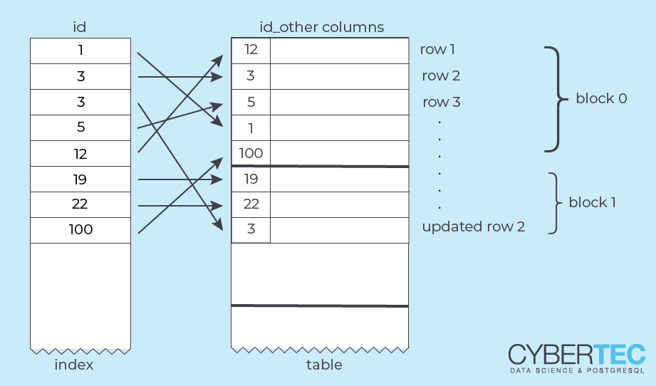
UPDATEPostgreSQL implements multiversioning by keeping the old version of the table row in the table – an UPDATE adds a new row version (“tuple”) of the row and marks the old version as invalid.
In many respects, an UPDATE in PostgreSQL is not much different from a DELETE followed by an INSERT.
This has a lot of advantages:
ROLLBACK does not have to undo anything and is very fastBut it also has some disadvantages:
VACUUM)Essentially, UPDATE-heavy workloads are challenging for PostgreSQL. This is the area where HOT updates help. Since PostgreSQL v12, we can extend PostgreSQL to define alternative way to persist tables. zheap, which is currently work in progress, is an implementation that should handle UPDATE-heavy workloads better.
UPDATE exampleLet's create a simple table with 235 rows:
|
1 2 3 4 5 6 7 8 |
CREATE TABLE mytable ( id integer PRIMARY KEY, val integer NOT NULL ) WITH (autovacuum_enabled = off); INSERT INTO mytable SELECT *, 0 FROM generate_series(1, 235) AS n; |
This table is slightly more than one 8KB block long. Let's look at the physical address (“current tuple ID” or ctid) of each table row:
|
1 2 3 4 5 6 7 8 9 10 11 12 13 14 15 16 17 18 19 20 21 22 23 24 |
SELECT ctid, id, val FROM mytable; ctid | id | val ---------+-----+----- (0,1) | 1 | 0 (0,2) | 2 | 0 (0,3) | 3 | 0 (0,4) | 4 | 0 (0,5) | 5 | 0 ... (0,224) | 224 | 0 (0,225) | 225 | 0 (0,226) | 226 | 0 (1,1) | 227 | 0 (1,2) | 228 | 0 (1,3) | 229 | 0 (1,4) | 230 | 0 (1,5) | 231 | 0 (1,6) | 232 | 0 (1,7) | 233 | 0 (1,8) | 234 | 0 (1,9) | 235 | 0 (235 rows) |
The ctid consists of two parts: the “block number”, starting at 0, and the “line pointer” (tuple number within the block), starting at 1.
So the first 226 rows fill block 0, and the last 9 are in block 1.
Let's run an UPDATE:
|
1 2 3 4 5 6 7 8 9 10 11 12 |
UPDATE mytable SET val = -1 WHERE id = 42; SELECT ctid, id, val FROM mytable WHERE id = 42; ctid | id | val --------+----+----- (1,10) | 42 | -1 (1 row) |
The new row version was added to block 1, which still has free space.
To understand HOT, let's recapitulate the layout of a table page in PostgreSQL:
The array of “line pointers” is stored at the beginning of the page, and each points to an actual tuple. This indirect reference allows PostgreSQL to reorganize a page internally without changing the outside appearance.
A Heap Only Tuple is a tuple that is not referenced from outside the table block. Instead, a “forwarding address” (its line pointer number) is stored in the old row version:
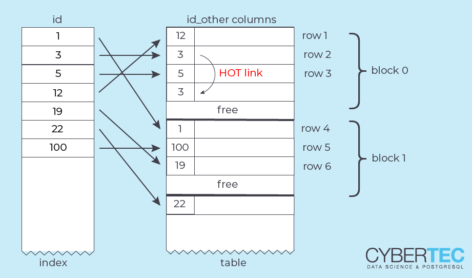
That only works if the new and the old version of the row are in the same block. The external address of the row (the original line pointer) remains unchanged. To access the heap only tuple, PostgreSQL has to follow the “HOT chain” within the block.
There are two main advantages of HOT updates:
VACUUM.If there are several HOT updates on a single row, the HOT chain grows longer. Now any backend that processes a block and detects a HOT chain with dead tuples (even a SELECT!) will try to lock and reorganize the block, removing intermediate tuples. This is possible, because there are no outside references to these tuples.This greatly reduces the need for VACUUM for UPDATE-heavy workloads.There are two conditions for HOT updates to be used:
The second condition is not obvious and is required by the current implementation of the feature.
fillfactor on tables to get HOT updatesYou can make sure that the second condition from above is satisfied, but how can you make sure that there is enough free space in table blocks? For that, we have the storage parameter fillfactor. It is a value between 10 and 100 and determines to which percentage INSERTs will fill a table block. If you choose a value less than the default 100, you can make sure that there is enough room for HOT updates in each table block.
The best value for fillfactor will depend on the size of the average row (larger rows need lower values) and the workload.
Note that setting fillfactor on an existing table will not rearrange the data, it will only apply to future INSERTs. But you can use VACUUM (FULL) or CLUSTER to rewrite the table, which will respect the new fillfactor setting.
There is a simple way to see if your setting is effective and if you get HOT updates:
|
1 2 3 4 |
SELECT n_tup_upd, n_tup_hot_upd FROM pg_stat_user_tables WHERE schemaname = 'myschema' AND relname = 'mytable'; |
This will show cumulative counts since the last time you called the function pg_stat_reset().
Check if n_tup_hot_upd (the HOT update count) grows about as fast as n_tup_upd (the update count) to see if you get the HOT updates you want.
Let's change the fillfactor for our table and repeat the experiment from above:
|
1 2 3 4 5 6 7 8 9 10 11 12 13 14 15 16 17 18 19 20 21 22 23 24 25 26 27 28 29 |
TRUNCATE mytable; ALTER TABLE mytable SET (fillfactor = 70); INSERT INTO mytable SELECT *, 0 FROM generate_series(1, 235); SELECT ctid, id, val FROM mytable; ctid | id | val ---------+-----+----- (0,1) | 1 | 0 (0,2) | 2 | 0 (0,3) | 3 | 0 (0,4) | 4 | 0 (0,5) | 5 | 0 ... (0,156) | 156 | 0 (0,157) | 157 | 0 (0,158) | 158 | 0 (1,1) | 159 | 0 (1,2) | 160 | 0 (1,3) | 161 | 0 ... (1,75) | 233 | 0 (1,76) | 234 | 0 (1,77) | 235 | 0 (235 rows) |
This time there are fewer tuples in block 0, and some space is still free.
Let's run the UPDATE again and see how it looks this time:
|
1 2 3 4 5 6 7 8 9 10 11 12 |
UPDATE mytable SET val = -1 WHERE id = 42; SELECT ctid, id, val FROM mytable WHERE id = 42; ctid | id | val ---------+----+----- (0,159) | 42 | -1 (1 row) |
The updated row was written into block 0 and was a HOT update.
HOT updates are the one feature that can enable PostgreSQL to handle a workload with many UPDATEs.
In UPDATE-heavy workloads, it can be a life saver to avoid indexing the updated columns and setting a fillfactor of less than 100.
If you are interested in performance measurements for HOT updates, look at this article by Kaarel Moppel.
In order to receive regular updates on important changes in PostgreSQL, subscribe to our newsletter, or follow us on Twitter, Facebook, or LinkedIn.
SQL and PostgreSQL are perfect tools to analyze data. However, they can also be used to create sample data which has to possess certain statistical properties. One thing many people need quite often is a normal distribution. The main question therefore is: How can I create this kind of sample data?
The first thing you have to do is to enable the tablefunc extension, which is actually quite simple to do:
|
1 2 |
test=# CREATE EXTENSION tablefunc; CREATE EXTENSION |
“tablefunc” is there by default if “postgresql-contrib” has been installed. Once the module has been enabled the desired functions will already be there:
|
1 2 3 4 5 6 |
test=# df *normal_rand* List of functions Schema | Name | Result data type | Argument data types | Type --------+-------------+------------------------+---------------------------------------------+------ public | normal_rand | SETOF double precision | integer, double precision, double precision | func (1 row) |
The normal_rand function takes 3 parameters:
If you want to run the function, you can simply put it into the FROM-clause and pass the desired
parameters to the function:
|
1 2 3 4 5 6 7 8 9 10 11 12 13 14 15 16 |
test=# SELECT row_number() OVER () AS id, x FROM normal_rand(10, 5, 1) AS x ORDER BY 1; id | x ----+-------------------- 1 | 4.332941804386073 2 | 4.905662881624426 3 | 3.661038976418651 4 | 6.0087510163144415 5 | 4.934066454147052 6 | 5.909371874123449 7 | 5.016528121699469 8 | 4.640932937572484 9 | 7.695984939477616 10 | 5.647677569953539 (10 rows) |
In this case 10 rows were created. The average value is 5 and the standard deviation has been set to 1. At first glance the data looks ok.
Let us test the function and see if it really does what it promises. 10 rows won't be enough for that so I decided to repeat the test with more data:
|
1 2 3 4 5 6 |
test=# SELECT count(*), avg(x), stddev(x) FROM normal_rand(1000000, 5, 1) AS x; count | avg | stddev ---------+-------------------+------------------- 1000000 | 5.000273593685213 | 1.000627143792761 (1 row) |
Running the test with 1 million rows clearly shows that the output is perfect. The average value is very close to 5 and the same holds true for the standard deviation. You can therefore safely use the output to handle all your calculations.
Once you have a Gaussian distribution, you can nicely turn it into some other distribution of your choice or simply built on this data.
If you want to know more about data, statistical distributions and so on you can check out one of our other posts about fraud detection.
Is it Postgre, PostGreSQL, Postgres or PostgreSQL? We have all seen a couple of wrong ways to spell “PostgreSQL”. The question therefore is: How can one find data even if there are typos? In PostgreSQL there are various solutions to the problem. Depending on what kind of search you need you can choose between various methods.
Before we get started it is necessary to compile some sample data:
|
1 2 3 4 5 6 7 8 9 10 11 12 |
CREATE EXTENSION citext; CREATE TABLE t_database ( real_name citext ); INSERT INTO t_database VALUES ('PostgreSQL'), ('Postgres'), ('PostGreSQL'), ('postgres'), ('DB2'), ('DB/2 LUW'), ('DB/2'), ('IBM DB2'), ('Oracle'), ('MS SQL Server'), ('Microsoft SQL Server'); |
All we have here is the name of some database along with a handful of different spellings and typos.
There is one common thing people need quite frequently: Case-insensitive search. Of course one can work around this problem using “upper” and “lower” but in many cases this is simply less convenient than it should be. In addition to that developers have to keep these things in mind at all times which can lead to bugs.
Fortunately, there is a more simplistic solution available: The “citext” datatype (as provided by the “citext” extension) can handle case-insensitive comparisons. The following example shows how it works:
|
1 2 3 4 5 6 |
test=# SELECT * FROM t_database WHERE real_name = 'postgresql'; real_name ------------ PostgreSQL PostGreSQL (2 rows) |
As you can see, the data in the table is elegantly preserved. Just the comparison function is a bit more relaxed. Solving the case-sensitivity issue on the data type level is really nice and makes life a lot easier for all software making use of the database. The citext extension is available on all public clouds including Amazon AWS, Microsoft Azure and so on.
LIKE and ILIKE are the classical means to do similarity search in PostgreSQL:
|
1 2 3 4 5 6 7 8 |
test=# SELECT * FROM t_database WHERE real_name ILIKE 'postgr%'; real_name ------------ PostgreSQL Postgres PostGreSQL postgres (4 rows) |
As you can see, we can find all incarnations of PostgreSQL in an easy way. However, LIKE and ILIKE have a major limitation: One has to know quite a lot about the spelling of things you are looking for. In my example we needed at string that contained “postgr” - but what if somebody had used “BostgreSQL”? We would not have found anything. In other words: LIKE and ILIKE are good but in many cases these two keywords are not sufficient to find what is really needed.
Trigrams are an additional way, provided by PostgreSQL, to handle similarity search and are more suitable to handle typos. To use trigrams one has to install the extension:
|
1 2 |
test=# CREATE EXTENSION pg_trgm; CREATE EXTENSION |
The trigram extension provides us with the distance operator. It helps us to find similar strings. Let us give it a try: Support we want to search for “db3” because we did not quite understand that the IBM product is actually called “DB2”. Here is what happens:
|
1 2 3 4 5 6 7 8 9 10 11 12 13 14 15 16 17 |
test=# SELECT real_name <-> 'db3', * FROM t_database ORDER BY real_name <-> 'db3'; ?column? | real_name ------------+---------------------- 0.6666666 | DB2 0.71428573 | DB/2 0.8 | IBM DB2 0.8181818 | DB/2 LUW 1 | Oracle 1 | MS SQL Server 1 | PostgreSQL 1 | Microsoft SQL Server 1 | Postgres 1 | PostGreSQL 1 | postgres (11 rows) |
We can sort by distance which ideally gives us the string closest to what we are searching for. As you can see “DB2” and “DB/2” come out on top which is exactly the way it should be. Of course pg_trgm is not the holy grail and should be used with caution. However, it is one way to tackle the problems caused by wrong data.
While pg_trgm is useful is you are looking for names, addresses and so on full text search has a slightly different purpose. The goal is to look for certain words in text. Here is an example:
|
1 2 3 4 5 6 7 |
test=# SELECT real_name, to_tsvector(real_name) FROM t_database WHERE to_tsvector(real_name) @@ to_tsquery('server & microsoft'); real_name | to_tsvector ----------------------+---------------------------------- Microsoft SQL Server | 'microsoft':1 'server':3 'sql':2 (1 row) |
We are looking for the words “server” and “microsoft”. Naturally one row is returned. What is noteworthy here is that the order of words can be swapped. We simply want to make sure that all words are in the string - for now order does not matter.
Full text search in PostgreSQL is quite powerful and it offers a variety of additional features which are way beyond the scope of this posting.
However, what can we do if the order of words does matter? The answer is “phrase search”: PostgreSQL allows you to specify in which order words have to appear:
|
1 2 3 4 5 6 7 |
test=# SELECT real_name, to_tsvector(real_name) FROM t_database WHERE to_tsvector(real_name) @@ to_tsquery('microsoft <-> sql'); real_name | to_tsvector ----------------------+---------------------------------- Microsoft SQL Server | 'microsoft':1 'server':3 'sql':2 (1 row) |
In this case we want “microsoft” followed by “sql”. PostgreSQL will return the right row. However, what if we look for “microsoft” followed by “server”? In this case things will fail because there happens to be a word in between which is not allowed:
|
1 2 3 4 5 6 |
test=# SELECT real_name, to_tsvector(real_name) FROM t_database WHERE to_tsvector(real_name) @@ to_tsquery('microsoft <-> server'); real_name | to_tsvector -----------+------------- (0 rows) |
Fortunately, PostgreSQL (https://www.postgresql.org/docs/current/functions-textsearch.html) has a feature indicating how far things are allowed to be apart. The following listing shows how this works:
|
1 2 3 4 5 6 7 |
test=# SELECT real_name, to_tsvector(real_name) FROM t_database WHERE to_tsvector(real_name) @@ to_tsquery('microsoft <2> server'); real_name | to_tsvector ----------------------+---------------------------------- Microsoft SQL Server | 'microsoft':1 'server':3 'sql':2 (1 row) |
PostgreSQL has many options to handle fuzzy search. There are many more things out there (such as pgsimilarity) which can be used to make our lives easier. One of the things people are often not aware of is the fact that full text search and indexing can also have an impact on the optimal VACUUM policy. Check out my posting about the “GIN pending list” to learn more.