
PostgreSQL v14 has new connection statistics in pg_stat_database. In this article, I want to explore one application for them: estimating the correct size for a connection pool.
Commit 960869da080 introduced some new statistics to pg_stat_database:
session_time: total time spent by sessions in the databaseactive_time: time spent executing SQL statements in the databaseidle_in_transaction_time: time spent idle in a transaction in the databasesessions: total number of sessions established to the databasesessions_abandoned: number of sessions to the database that were terminated by lost client connectionssessions_fatal: number of sessions to the database terminated by fatal errorssessions_killed: number of sessions to the database killed by an operatorSome applications are obvious: for example, you may want to keep the number of fatal errors or operator interventions low, or you may want to fix your application to properly close database connections.
But I want to show you another, less obvious, application for these statistics.
In the following, I assume that the application connects to the database with a single database user. That means that there will be one connection pool per database.
If you use session level connection pooling, a client gets a session from the pool for the whole duration of the database session. In this case, sizing the connection pool is simple: the pool has to be large enough to accommodate the maximum number of concurrent sessions. The number of connections to a database is available in numbackends in pg_stat_database, and many monitoring systems capture this value. Session level pooling is primarily useful if the client's database connections are short.
However, it is normally more efficient to use transaction level connection pooling. In this mode, a client gets a session only for the duration of a database transaction. The advantage is that multiple clients can share the same pooled session. Sharing reduces the required number of connections in the pool. Having few database connections is a good thing, because it reduces contention inside the database and limits the danger of overloading the CPU or storage subsystem.
Of course, transaction level pooling makes it more difficult to determine the correct size of the connection pool.
The ideal size for a connection pool is
In my article about max_connections, I established the following upper limit for the number of connections:
|
1 2 |
connections < min(num_cores, parallel_io_limit) / (session_busy_ratio * avg_parallelism) |
Where
num_cores is the number of cores availableparallel_io_limit is the number of concurrent I/O requests your storage subsystem can handlesession_busy_ratio is the fraction of time that the connection is active executing a statement in the databaseavg_parallelism is the average number of backend processes working on a single query.Now all these numbers are easy to determine – that is, all except for session_busy_ratio.
With the new database statistics, that task becomes trivial:
|
1 2 3 4 5 |
SELECT datname, active_time / (active_time + idle_in_transaction_time) AS session_busy_ratio FROM pg_stat_database WHERE active_time > 0; |
The new database statistics in PostgreSQL v14 make it easier to get an estimate for the safe upper limit for the size of a connection pool. To learn more about connection pools and authentication, see my post on pgbouncer.
In order to receive regular updates on important changes in PostgreSQL, subscribe to our newsletter, or follow us on Twitter, Facebook, or LinkedIn.
Just like in most databases, in PostgreSQL a trigger is a way to automatically respond to events. Maybe you want to run a function if data is inserted into a table. Maybe you want to audit the deletion of data, or simply respond to some UPDATE statement. That is exactly what a trigger is good for. This post is a general introduction to triggers in PostgreSQL. It is meant to be a tutorial for people who want to get started programming them.
Writing a trigger is easy. The first important thing you will need is a table. A trigger is always associated with a table:
|
1 2 3 4 5 6 7 8 9 10 11 12 13 14 15 |
test=# CREATE TABLE t_temperature ( id serial, tstamp timestamptz, sensor_id int, value float4 ); CREATE TABLE test=# d t_temperature Table 'public.t_temperature' Column | Type | Collation | Nullable | Default -----------+--------------------------+-----------+----------+------------------------------------------- id | integer | | not null | nextval('t_temperature_id_seq'::regclass) tstamp | timestamp with time zone | | | sensor_id | integer | | | value | real | | | |
The goal of this example is to check the values inserted and silently “correct” them if we think that the data is wrong. For the sake of simplicity, all values below zero will be set to -1.
If you want to define a trigger, there are two things which have to be done:
In the following section you will be guided through that process.
Before we get started, let’s first take a look at CREATE TRIGGER:
|
1 2 3 4 5 6 7 8 9 10 11 12 13 14 15 16 17 18 19 20 21 |
test=# h CREATE TRIGGER Command: CREATE TRIGGER Description: define a new trigger Syntax: CREATE [ OR REPLACE ] [ CONSTRAINT ] TRIGGER name { BEFORE | AFTER | INSTEAD OF } { event [ OR ... ] } ON table_name [ FROM referenced_table_name ] [ NOT DEFERRABLE | [ DEFERRABLE ] [ INITIALLY IMMEDIATE | INITIALLY DEFERRED ] ] [ REFERENCING { { OLD | NEW } TABLE [ AS ] transition_relation_name } [ ... ] ] [ FOR [ EACH ] { ROW | STATEMENT } ] [ WHEN ( condition ) ] EXECUTE { FUNCTION | PROCEDURE } function_name ( arguments ) where event can be one of: INSERT UPDATE [ OF column_name [, ... ] ] DELETE TRUNCATE URL: https://www.postgresql.org/docs/15/sql-createtrigger.html |
URL: https://www.postgresql.org/docs/15/sql-createtrigger.html
The first thing you can see is that a trigger can be executed BEFORE or AFTER. But “before” and “after” what? Well, if you insert a row, you can call a function before or after its insertion. If you call the function before the actual insertion, you can modify the row before it finds its way to the table. In case of an AFTER trigger, the trigger function can already see the row which has just been inserted - the data is already inserted.
The following image shows where to insert a trigger:
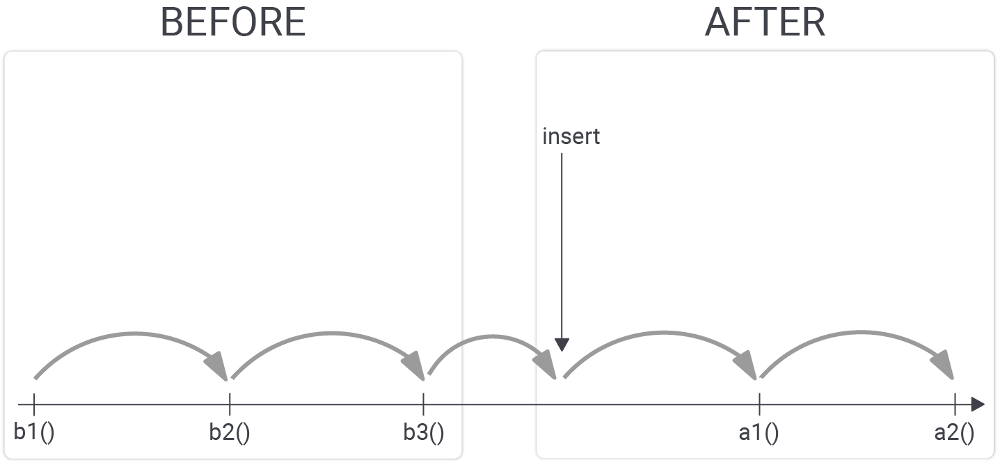
Basically, you can have as many BEFORE and as many AFTER triggers as you like. The important thing is that the execution order of the triggers is deterministic (since PostgreSQL 7.3). Triggers are always executed ordered by name. In other words, PostgreSQL will execute all BEFORE triggers in alphabetical order, do the actual operation, and then execute all AFTER triggers in alphabetical order.
Execution order is highly important, since it makes sure that your code runs in a deterministic order. To see how this plays out, let’s take a look at a practical example.
As stated before, we want to change the value being inserted in case it is negative. To do that, I have written an easy to understand function:
|
1 2 3 4 5 6 7 8 9 10 11 12 13 14 15 |
CREATE OR REPLACE FUNCTION f_temp () RETURNS trigger AS $ DECLARE BEGIN RAISE NOTICE 'NEW: %', NEW; IF NEW.value < 0 THEN NEW.value := -1; RETURN NEW; END IF; RETURN NEW; END; $ LANGUAGE 'plpgsql'; |
What we see here is this NEW variable. It contains the current row the trigger has been fired for. We can easily access and modify this variable, which in turn will modify the value which ends up in the table.
NOTE: If the function returns NEW, the row will be inserted as expected. However, if you return NULL, the operation will be silently ignored. In case of a BEFORE trigger the row will not be inserted.
The next step is to create a trigger and tell it to call this function:
|
1 2 3 |
CREATE TRIGGER xtrig BEFORE INSERT ON t_temperature FOR EACH ROW EXECUTE PROCEDURE f_temp(); |
Our trigger will only fire on INSERT (shortly before it happens). What is also noteworthy here: In PostgreSQL, a trigger on a table can fire for each row or for each statement. In most cases, people use row level triggers and execute a function for each row modified.
Once the code has been deployed we can already test it:
|
1 2 3 4 5 6 7 8 9 10 11 12 13 |
test=# INSERT INTO t_temperature (tstamp, sensor_id, value) VALUES ('2021-05-04 13:23', 1, -196.4), ('2021-06-03 12:32', 1, 54.5) RETURNING *; NOTICE: NEW: (4,'2021-05-04 13:23:00+02',1,-196.4) NOTICE: NEW: (5,'2021-06-03 12:32:00+02',1,54.5) id | tstamp | sensor_id | value ----+------------------------+-----------+------- 4 | 2021-05-04 13:23:00+02 | 1 | -1 5 | 2021-06-03 12:32:00+02 | 1 | 54.5 (2 rows) INSERT 0 2 |
In this example two rows are inserted. One row is modified - the second one is taken as it is. In addition to that, our trigger issues two log messages so that we can see the content of NEW.
The previous example focuses on INSERT and therefore the NEW variable is readily available. However, if you want to write a trigger handling UPDATE and DELETE, the situation is quite different. Depending on the operation, different variables are available:
In other words: If you want to write a trigger for UPDATE, you have full access to the old as well as the new row. In case of DELETE you can see the row which is about to be deleted.
So far we have seen NEW and OLD - but there is more.
PostgreSQL offers a variety of additional predefined variables which can be accessed inside a trigger function. Basically, the function knows when it has been called, what kind of operation it is called for, and so on.
Let's take a look at the following code snippet:
|
1 2 3 4 5 6 7 8 9 10 11 12 13 14 15 16 17 18 19 20 21 22 23 24 25 26 27 28 |
CREATE OR REPLACE FUNCTION f_predefined () RETURNS trigger AS $ DECLARE BEGIN RAISE NOTICE 'NEW: %', NEW; RAISE NOTICE 'TG_RELID: %', TG_RELID; RAISE NOTICE 'TG_TABLE_SCHEMA: %', TG_TABLE_SCHEMA; RAISE NOTICE 'TG_TABLE_NAME: %', TG_TABLE_NAME; RAISE NOTICE 'TG_RELNAME: %', TG_RELNAME; RAISE NOTICE 'TG_OP: %', TG_OP; RAISE NOTICE 'TG_WHEN: %', TG_WHEN; RAISE NOTICE 'TG_LEVEL: %', TG_LEVEL; RAISE NOTICE 'TG_NARGS: %', TG_NARGS; RAISE NOTICE 'TG_ARGV: %', TG_ARGV; RAISE NOTICE ' TG_ARGV[0]: %', TG_ARGV[0]; RETURN NEW; END; $ LANGUAGE 'plpgsql'; CREATE TRIGGER trig_predefined BEFORE INSERT ON t_temperature FOR EACH ROW EXECUTE PROCEDURE f_predefined('hans'); INSERT INTO t_temperature (tstamp, sensor_id, value) VALUES ('2025-02-12 12:21', 2, 534.4); |
As you can see, there are various TG_* variables. Let’s take a look at them and see what they contain:
Let's run the code shown in the previous listing and see what happens:
|
1 2 3 4 5 6 7 8 9 10 11 12 |
NOTICE: NEW: (8,'2025-02-12 12:21:00+01',2,534.4) NOTICE: TG_RELID: 98399 NOTICE: TG_TABLE_SCHEMA: public NOTICE: TG_TABLE_NAME: t_temperature NOTICE: TG_RELNAME: t_temperature NOTICE: TG_OP: INSERT NOTICE: TG_WHEN: BEFORE NOTICE: TG_LEVEL: ROW NOTICE: TG_NARGS: 1 NOTICE: TG_ARGV: [0:0]={hans} NOTICE: TG_ARGV[0]: hans NOTICE: NEW: (8,'2025-02-12 12:21:00+01',2,534.4) |
The trigger shows us exactly what's going on. That's important if you want to make your functions more generic. You can use the same function and apply it to more than just one table.
Triggers can do a lot more and it certainly makes sense to dig into this subject deeper to understand the inner workings of this important technique.
If you want to learn more about important features of PostgreSQL, you might want to check out one of my posts about sophisticated temporary tables which can be found here.
PostgreSQL query optimization with CREATE STATISTICS is an important topic. Usually, the PostgreSQL optimizer (query planner) does an excellent job. This is not only true for OLTP but also for data warehousing. However, in some cases the optimizer simply lacks the information to do its job properly. One of these situations has to do with cross-column correlation. Let’s dive in and see what that means.
Often data is not correlated at all. The color of a car might have nothing to do with the amount of gasoline consumed. You wouldn’t expect a correlation between the number of dogs in China and the price of coffee. However, sometimes there is indeed a correlation between columns which can cause a problem during query optimization.
Why is that the case? In PostgreSQL, statistics are stored for each column. PostgreSQL knows about the number of distinct entries, the distribution of data, and so on - by default it does NOT know how values relate to each other. Some examples: you know that age and height correlate (babies are not born 6 ft tall), you know that “country” and “language” spoken are usually correlated. However, the PostgreSQL query planner does not know that.
The solution to the problem is extended statistics (“CREATE STATISTICS”).
Let us create some same sample data:
|
1 2 3 4 5 6 7 8 9 10 |
test=# CREATE TABLE t_test (id serial, x int, y int, z int); CREATE TABLE test=# INSERT INTO t_test (x, y, z) SELECT id % 10000, (id % 10000) + 50000, random() * 100 FROM generate_series(1, 10000000) AS id; INSERT 0 10000000 test=# ANALYZE ; ANALYZE |
What we do here is to create 10 million rows. The magic is in the first two columns: We see that the “y” is directly related to “x” - we simply add 50.000 to make sure that the data is perfectly correlated.
In the next example we will take a look at a simple query and see how PostgreSQL handles statistics. To make the plan more readable and the statistics more understandable, we will turn parallel queries off:
|
1 2 3 4 5 6 7 8 9 10 |
test=# SET max_parallel_workers_per_gather TO 0; SET test=# explain SELECT x, y, count(*) FROM t_test GROUP BY 1, 2; QUERY PLAN ------------------------------------------------------------------------ HashAggregate (cost=741567.03..829693.58 rows=1000018 width=16) Group Key: x, y Planned Partitions: 32 -> Seq Scan on t_test (cost=0.00..154056.75 rows=10000175 width=8) (4 rows) |
What we see here is highly interesting: The planner assumes that roughly one million rows will be returned. However, this is not true - as the following listing clearly shows:
|
1 2 3 4 5 6 7 8 9 10 11 12 |
test=# explain analyze SELECT x, y, count(*) FROM t_test GROUP BY 1, 2; QUERY PLAN ---------------------------------------------------------------------------------- HashAggregate (cost=741567.03..829693.58 rows=1000018 width=16) (actual time=2952.991..2954.460 rows=10000 loops=1) Group Key: x, y Planned Partitions: 32 Batches: 1 Memory Usage: 2577kB -> Seq Scan on t_test (cost=0.00..154056.75 rows=10000175 width=8) (actual time=0.036..947.466 rows=10000000 loops=1) Planning Time: 0.081 ms Execution Time: 2955.077 ms (6 rows) |
As you can see, the planner greatly overestimates the number of groups. Why is that the case? The planner simply multiplies the number of entries in “x” with the number of entries in “y”. So 10.000 x 10.000 makes one million. Note that the result is not precise, because PostgreSQL is using estimates here. A wrong estimate can greatly reduce performance and cause serious issues.
Therefore, a solution is needed: “CREATE STATISTICS” allows you to create statistics about the expected number of distinct entries, given a list of columns:
|
1 2 3 4 |
test=# CREATE STATISTICS mygrp (ndistinct) ON x, y FROM t_test; CREATE STATISTICS test=# ANALYZE t_test; ANALYZE |
In this case, statistics for x and y are needed. Refreshing those statistics can easily be done with ANALYZE. PostgreSQL will automatically maintain those extended statistics for you.
The key question is: What does it mean for our estimates? Let us run the same query again and inspect the estimates:
|
1 2 3 4 5 6 7 |
test=# explain SELECT x, y, count(*) FROM t_test GROUP BY 1, 2; QUERY PLAN ----------------------------------------------------------------------- HashAggregate (cost=229052.55..229152.39 rows=9984 width=16) Group Key: x, y -> Seq Scan on t_test (cost=0.00..154053.60 rows=9999860 width=8) (3 rows) |
Wow, 9984 groups. We are right on target.
If your queries are more complex, such improvements can have a huge impact on performance and speed things up considerably.
What you have seen in this example is “CREATE STATISTICS” using the “ndistinct” method. In the case of GROUP BY, this method is what you need. If you want to speed up standard WHERE clauses, you might want to dig into the “dependencies” method to improve statistics accuracy.
If you want to learn more about query optimization in general, you might want to check out my blog post about GROUP BY. It contains some valuable tips on how to run analytical queries faster.
Also, If you have any comments, feel free to share them in the Disqus section below. If there are any topics you are especially interested in, feel free to share them as well. We can certainly cover your topics of interest in future articles.
Our PostgreSQL 24x7 support team recently received a request from one of our customers who was facing a performance problem. The solution to the problem could be found in the way PostgreSQL handles query optimization (specifically, statistics). So I thought it would be nice to share some of this knowledge with my beloved readers. The topic of this post is therefore: What kinds of statistics does PostgreSQL store, and where can they be found? Let’s dive in and find out.
Before we dig into PostgreSQL optimization and statistics, it makes sense to understand how PostgreSQL runs a query. The typical process works as follows:
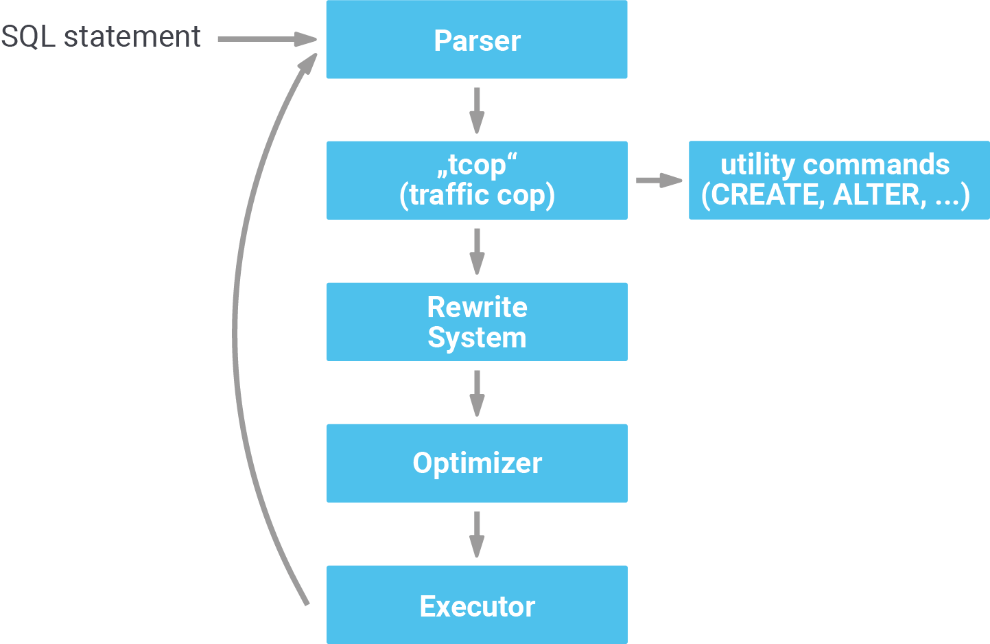
First, PostgreSQL parses the query. Then, the traffic cop separates the utility commands (ALTER, CREATE, DROP, GRANT, etc.) from the rest. After that, the entire thing goes through the rewrite system, which is in charge of handling rules and so on.
Next comes the optimizer - which is supposed to produce the best plan possible. The plan can then be executed by the executor. The main question now is: What does the optimizer do to find the best possible plan? In addition to many mathematical transformations, it uses statistics to estimate the number of rows involved in a query. Let’s take a look and see:
|
1 2 3 4 5 6 7 8 |
test=# CREATE TABLE t_test AS SELECT *, 'hans'::text AS name FROM generate_series(1, 1000000) AS id; SELECT 1000000 test=# ALTER TABLE t_test ALTER COLUMN id SET STATISTICS 10; ALTER TABLE test=# ANALYZE; ANALYZE |
I have created 1 million rows and told the system to calculate statistics for this data. To make things fit onto my website, I also told PostgreSQL to reduce the precision of the statistics. By default, the statistics target is 100. However, I decided to use 10 here, to make things more readable - but more on that later.
Now let’s run a simple query:
|
1 2 3 4 5 6 |
test=# explain SELECT * FROM t_test WHERE id < 150000; QUERY PLAN --------------------------------------------------------------- Seq Scan on t_test (cost=0.00..17906.00 rows=145969 width=9) Filter: (id < 150000) (2 rows) |
What we see here is that PostgreSQL expected 145.000 rows to be returned by the sequential scan. This information is highly important because if the system knows what to expect, it can adjust its strategy accordingly (index, no index, etc.). In my case there are only two choices:
|
1 2 3 4 5 |
test=# explain SELECT * FROM t_test WHERE id < 1; QUERY PLAN --------------------------------------- ------------------------ Gather (cost=1000.00..11714.33 rows=1000 width=9) Workers Planned: 2 -> Parallel Seq Scan on t_test (cost=0.00..10614.33 rows=417 width=9) Filter: (id < 1) (4 rows) |
All I did was to change the number in the WHERE-clause and all of a sudden, the plan has changed. The first query expected a fairly big result set; therefore it was not useful to fire up parallelism, because collecting all those rows in the gather node would have been too expensive. In the second example, the seq scan rarely yields rows - so a parallel query makes sense.
To find the best strategy, PostgreSQL relies on statistics to give the optimizer an indication of what to expect. The better the statistics, the better PostgreSQL can optimize the query.
If you want to see which kind of data PostgreSQL uses, you can take a look at pg_stats which is a view that displays statistics to the user. Here is the content of the view:
|
1 2 3 4 5 6 7 8 9 10 11 12 13 14 15 16 17 18 |
test=# d pg_stats View 'pg_catalog.pg_stats' Column | Type | Collation | Nullable | Default ------------------------+----------+-----------+----------+--------- schemaname | name | | | tablename | name | | | attname | name | | | inherited | boolean | | | null_frac | real | | | avg_width | integer | | | n_distinct | real | | | most_common_vals | anyarray | | | most_common_freqs | real[] | | | histogram_bounds | anyarray | | | correlation | real | | | most_common_elems | anyarray | | | most_common_elem_freqs | real[] | | | elem_count_histogram | real[] | | | |
Let's go through this step-by-step and dissect what kind of data the planner can use:
WHERE col IS NULL” or “WHERE col IS NOT NULL”Finally, there are some entries related to arrays - but let’s not worry about those for the moment. Rather, let’s take a look at some sample content:
|
1 2 3 4 5 6 7 8 9 10 11 12 13 14 15 16 17 18 19 20 21 22 23 24 25 26 27 28 29 30 31 32 33 |
test=# x Expanded display is on. test=# SELECT * FROM pg_stats WHERE tablename = 't_test'; -[ RECORD 1 ]----------+--------------------------------------------------------------------------- schemaname | public tablename | t_test attname | id inherited | f null_frac | 0 avg_width | 4 n_distinct | -1 most_common_vals | most_common_freqs | histogram_bounds | {47,102906,205351,301006,402747,503156,603102,700866,802387,901069,999982} correlation | 1 most_common_elems | most_common_elem_freqs | elem_count_histogram | -[ RECORD 2 ]----------+--------------------------------------------------------------------------- schemaname | public tablename | t_test attname | name inherited | f null_frac | 0 avg_width | 5 n_distinct | 1 most_common_vals | {hans} most_common_freqs | {1} histogram_bounds | correlation | 1 most_common_elems | most_common_elem_freqs | elem_count_histogram | |
In this listing, you can see what PostgreSQL knows about our table. In the “id” column, the histogram part is most important: “{47,102906,205351,301006,402747,503156,603102,700866,802387,901069,999982}”. PostgreSQL thinks that the smallest value is 47. 10% are smaller than 102906, 20% are expected to be smaller than 205351, and so on. What is also interesting here is the n_distinct: -1 basically means that all values are different. This is important if you are using GROUP BY. In the case of GROUP BY the optimizer wants to know how many groups to expect. n_distinct is used in many cases to provide us with that estimate.
In the case of the “name” column we can see that “hans” is the most frequent value (100%). That’s why we don’t get a histogram.
Of course, there is a lot more to say about how the PostgreSQL optimizer operates. However, to start out with, it is very useful to have a basic understanding of the way Postgres uses statistics.
In general, PostgreSQL generates statistics pretty much automatically. The autovacuum daemon takes care that statistics are updated on a regular basis. Statistics are the fuel needed to optimize queries properly. That’s why they are super important.
If you want to create statistics manually, you can always run ANALYZE. However, in most use cases, autovacuum is just fine.
If you want to learn more about query optimization in general you might want to check out my blog post about GROUP BY. It contains some valuable tips to run analytical queries faster.
Also, If you have any comments, feel free to share them in the Disqus section below. If there are any topics you are especially interested in, feel free to share them as well. We can certainly cover them in future articles.
Recently a colleague in our sales department asked me for a way to partition an area of interest spatially. He wanted to approximate customer potential and optimize our sales strategies respective trips.
Furthermore he wanted the resulting regions to be created around international airports first, and then intersected by potential customer locations, in order to support a basic ranking. Well, I thought this would be a good opportunity to experiment with lesser-known PostGIS functions ????.
In our case, customer locations could be proxied by major cities.
It's also worth mentioning that I only used freely available datasets for this demo.
Here is the basic structure of the process:
Our sales team will kick off their trips from international airports in Germany, so we require locations and classifications of airports from Germany. Airports can be extracted from OpenStreetMap datasets filtering osm_points by Tag:aeroway=aerodrome. Alternatively, any other data source containing the most recent airport locations and classifications is welcome. For our demo, I decided to give a freely available csv from “OurAirports” a chance ????.
In addition, I used OpenStreetMap datasets to gather both spatial and attributive data for cities located in Germany. To do so, I downloaded the most recent dataset covering Germany from Geofabrik and subsequently triggered the PostGIS import utilizing osm2pgsql. Please checkout my blogpost on this topic to get more details on how to accomplish this easily.
At the end of this article, you will find data structures for airports, osm_points and osm_polygons (country border). These are the foundation for our analysis.
Let’s start with cities and filter osm_points by place to retrieve only the major cities and towns.
|
1 2 3 4 5 6 |
SELECT planet_osm_point.name, planet_osm_point.way, planet_osm_point.tags -> 'population' :: text AS population, planet_osm_point.place FROM osmtile_germany.planet_osm_point WHERE planet_osm_point.place = ANY ( array [ 'city' :: text, 'town' :: text] ); |
Since we are only interested in international airports within Germany, let’s get rid of those tiny airports and heliports which are not relevant for our simple analysis.
|
1 2 3 4 5 6 7 8 9 10 11 12 13 |
WITH border AS ( SELECT way FROM osmtile_germany.planet_osm_polygon WHERE admin_level = '2' AND boundary = 'administrative') SELECT geom AS geom, NAME, type FROM osmtile_germany.airports, border WHERE type = 'large_airport' AND St_intersects(St_transform(airports.geom, 3857), border.way) |
Check out Figures 1 and 2 below to get an impression of what our core layers look like.
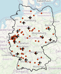
Figure 1 Major cities and international airports | 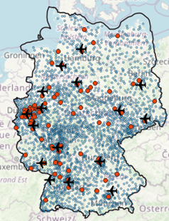 Figure 2 Major cities, towns and international airports |
So far, so good. It is time to start with our analysis by generating catchment areas around international airports first.
Instead of creating Voronoi polygons (Voronoi-Diagrams) using our preferred GIS-client, let us instead investigate how we can accomplish this task using only PostGIS’ functions.
|
1 2 3 4 5 6 7 8 9 10 11 12 13 14 15 |
WITH border AS ( SELECT way FROM osmtile_germany.planet_osm_polygon WHERE admin_level = '2' AND boundary = 'administrative'), airports AS ( SELECT St_collect(St_transform(geom, 3857)) AS geom FROM osmtile_germany.airports, border WHERE type = 'large_airport' AND St_intersects(St_transform(airports.geom, 3857), border.way)) SELECT (St_dump(St_voronoipolygons(geom))).geom FROM airports |
So how do we proceed? Let’s count the major cities by area as a proxy for potential customer counts, in order to rank the most interesting areas. As a reminder - major cities are only used here as a proxy for more detailed customer locations. They should be enriched by further datasets in order to more realistically approximate customer potential. Below, you see the final query which outputs major city count by polygon. Figure 4 represents the resulting Voronoi polygons extended by their major city counts. Query results and visualisation might be used as building blocks for optimizing customer acquisition in the future.
|
1 2 3 4 5 6 7 8 9 10 11 12 13 14 15 16 17 18 19 20 21 22 23 24 25 26 27 28 29 30 31 32 |
WITH border AS ( SELECT way FROM osmtile_germany.planet_osm_polygon WHERE admin_level = '2' AND boundary = 'administrative'), voronoi_polys AS ( SELECT (St_dump(St_voronoipolygons(St_collect(St_transform(geom, 3857))))).geom geom FROM osmtile_germany.airports, border WHERE type = 'large_airport' AND St_intersects(St_transform(airports.geom, 3857), border.way)) SELECT voronoi_polys.geom, a.NAME, b.majorcitycount FROM voronoi_polys, lateral ( SELECT NAME FROM osmtile_germany.airports, border WHERE St_intersects(voronoi_polys.geom, St_transform(osmtile_germany.airports.geom, 3857)) AND St_intersects(border.way, St_transform(osmtile_germany.airports.geom, 3857)) AND osmtile_germany.airports.type = 'large_airport' ) AS a, lateral ( SELECT count(*) majorcitycount FROM osmtile_germany.planet_osm_point WHERE place IN ('city') AND St_intersects(voronoi_polys.geom, osmtile_germany.planet_osm_point.way) ) AS b ORDER BY 3 DESC ; |
Today we started with some basic spatial analytics and took the opportunity to experiment with less known PostGIS functions.
Hopefully you enjoyed this session, and even more importantly, you’re now eager to play around with PostGIS and its rich feature set. It's just waiting to tackle your real-world challenges.
|
1 2 3 4 5 6 7 8 9 10 11 12 13 14 15 16 17 18 19 20 21 22 23 24 25 26 27 28 29 30 31 32 33 34 35 36 37 38 |
CREATE TABLE IF NOT EXISTS osmtile_germany.planet_osm_point ( osm_id bigint, name text, place text, tags hstore, way geometry(point, 3857) ); CREATE INDEX IF NOT EXISTS planet_osm_point_way_idx ON osmtile_germany.planet_osm_point USING gist (way); CREATE INDEX IF NOT EXISTS idx_osm_point_place ON osmtile_germany.planet_osm_point (place); CREATE TABLE IF NOT EXISTS osmtile_germany.airports ( gid serial NOT NULL CONSTRAINT airports_pkey PRIMARY KEY, type varchar(254), name varchar(254), geom geometry(point, 4326) ); CREATE INDEX IF NOT EXISTS airports_geom_idx ON osmtile_germany.airports USING gist (geom); CREATE INDEX IF NOT EXISTS airports_geom_3857_idx ON osmtile_germany.airports USING gist (St_transform (geom, 3857)); CREATE INDEX IF NOT EXISTS airports_type_index ON osmtile_germany.airports (type); CREATE TABLE IF NOT EXISTS osmtile_germany.planet_osm_polygon ( osm_id bigint, admin_level text, boundary text, name text, way geometry(Geometry, 3857) ); CREATE INDEX IF NOT EXISTS planet_osm_polygon_way_idx ON osmtile_germany.planet_osm_polygon USING gist (way); CREATE INDEX IF NOT EXISTS planet_osm_polygon_osm_id_idx ON osmtile_germany.planet_osm_polygon (osm_id); CREATE INDEX IF NOT EXISTS planet_osm_polygon_admin_level_boundary_index ON osmtile_germany.planet_osm_polygon (admin_level, boundary); |
PostgreSQL High-Availability has been one of the most dominant topics in the field for a long time. While there are many different approaches out there, Patroni seems to have become one of the most dominant solutions currently in use out there. Many database clusters run on Linux. However, we have seen some demand for a Microsoft Windows-based solution as well. The Patroni Environment Setup provides high availability for Windows.
While installing Patroni on Linux has become pretty simple, it is still an issue on Microsoft operating systems. There are simply too many parts that have to be in place to run Patroni and many people have found it hard to deploy Patroni.
PES is a graphical installer for Patroni on Windows which makes it really easy to deploy Patroni High-Availability. It takes care of all relevant components including:
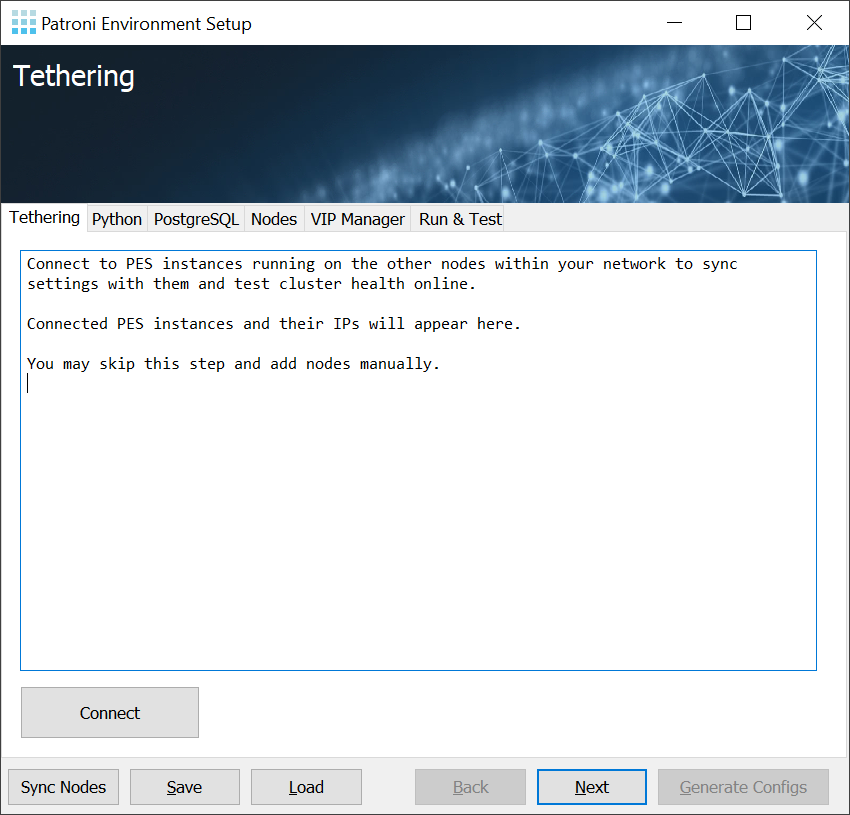
During the initialization step PES will try to find every instances already running over the network. Or the admin can skip this step and specify nodes and their roles manually.
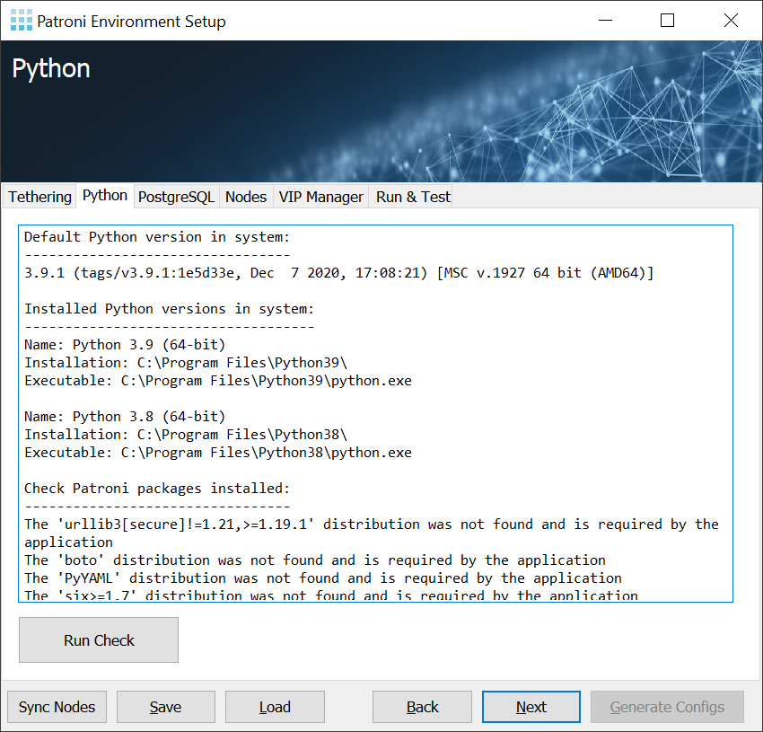
PES will stall what is already installed and what is not. All missing parts will be deployed with minimal effort.
One of the key issues is to configure more than one server at a time. PES makes it easy to solve this problem. Simply start PES on all nodes - the installer will then search for other running installers on the network and automatically exchange information.
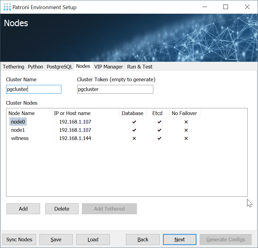
This greatly reduces the chances of configuration mistakes. If you want to build a reliable cluster it is essential that the etcd and Patroni configuration is not just correct but also consistent. By automatically exchanging information the risk of failure is reduced significantly.
PES is automatically going to configure all relevant services for you. It will make sure that ...
… are automatically started after a Windows reboot. The cluster is therefore ready for production use within minutes.
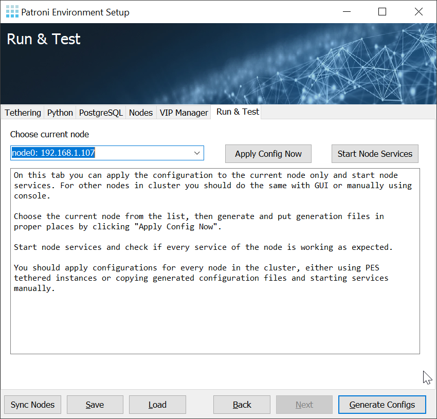
PES performs all necessary steps to provide you with a turnkey solution for PostgreSQL High-Availability and fault tolerance on Windows.
A database cluster consists of more than one machine. How does the application, therefore, know who is the current leader and which ones happen to be the replicas? The easiest solution to the problem is the introduction of service IPs. The core idea is to ensure that there is simply one IP all applications can connect to. The cluster itself will make sure that the service IP always points to the right server.
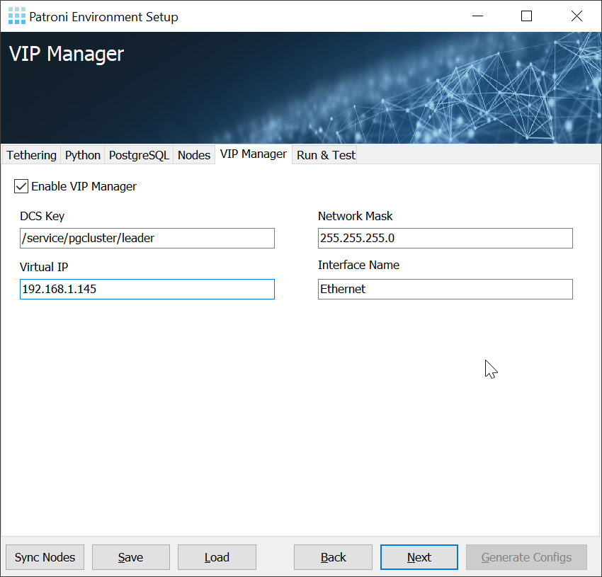
The tool capable of doing that on Windows and Linux is CYBERTEC vipmanager.
It checks etcd to figure out who the current leader is and makes sure the desired IPs are removed from a failed master and bound to the current leader.
The configuration is simple and easy to understand.
If you want to try out PES check out our GitHub repo or directly download our Windows installer (binary) here .
If you are looking for professional consulting services to setup PostgreSQL high-availability please check out our services.
Checkpoints are a core concept in PostgreSQL. However, many people don’t know what they actually are, nor do they understand how to tune checkpoints to reach maximum efficiency. This post will explain both checkpoints and checkpoint tuning, and will hopefully shed some light on these vital database internals.
Before we talk about checkpoints in more detail, it is important to understand how PostgreSQL writes data. Let’s take a look at the following image:
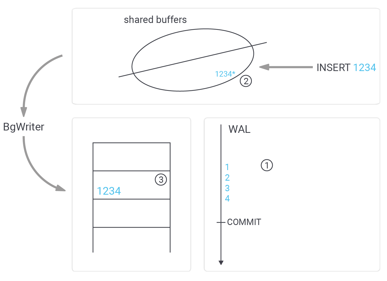
The most important thing is that we have to assume a crash could happen at any time. Why is that relevant? Well, we want to ensure that your database can never become corrupted. The consequence is that we cannot write data to the data files directly. Why is that? Suppose we wanted to write “1234” to the data file. What if we crashed after “12”? The result would be a broken row somewhere in the table. Perhaps index entries would be missing, and so on - we have to prevent that at all costs.
Therefore, a more sophisticated way to write data is necessary. How does it work? The first thing PostgreSQL does is to send data to the WAL ( = Write Ahead Log). The WAL is just like a paranoid sequential tape containing binary changes. If a row is added, the WAL might contain a record indicating that a row in a data file has to be changed, it might contain a couple of instructions to change the index entries, maybe an additional block has to be written and so on. It simply contains a stream of changes.
Once data is sent to the WAL, PostgreSQL will make changes to the cached version of a block in shared buffers. Note that data is still not in the datafiles. We now have got WAL entries as well as changes made to the shared buffers. If a read request comes in, it will not make it to the data files anyway - because the data is found in the cache.
At some point, those modified in-memory pages are written to disk by the background writer. The important thing here is that data might be written out of order, which is no problem. Bear in mind that if a user wants to read data, PostgreSQL will check shared buffers before asking the operating system for the block. The order in which dirty blocks are written is therefore not so relevant. It even makes sense to write data a bit later, to increase the odds of sending many changes to disk in a single I/O request.
However, we cannot write data to the WAL indefinitely. At some point, space has to be recycled. This is exactly what a checkpoint is good for.
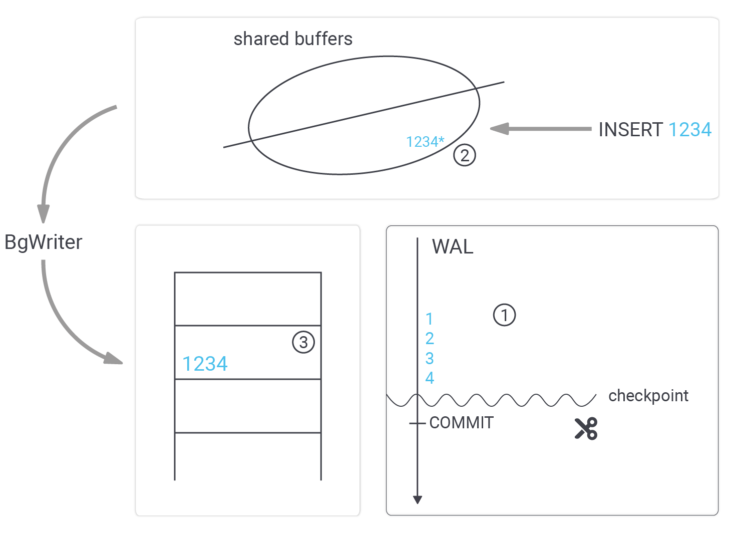
The purpose of a checkpoint is to ensure that all the dirty buffers created up to a certain point are sent to disk so that the WAL up to that point can be recycled. The way PostgreSQL does that is by launching a checkpointer process which writes those missing changes to the disk. However, this process does not send data to disk as fast as possible. The reason is that we want to flatten out the I/O curve to guarantee stable response times.
The parameter to control spreading the checkpoint is …
|
1 2 3 4 5 |
test=# SHOW checkpoint_completion_target; checkpoint_completion_target ------------------------------ 0.5 (1 row) |
The idea is that a checkpoint is finished halfway before the next checkpoint is expected to kick in. In real life, a value of 0.7 - 0.9 seems to be the best choice for most workloads, but feel free to experiment a bit.
NOTE: In PostgreSQL 14 this parameter will most likely not exist anymore. The hardcoded value will be 0.9 which will make it easier for end users.
The next important question is: When does a checkpoint actually kick in? There are some parameters to control this behavior:
|
1 2 3 4 5 |
test=# SHOW checkpoint_timeout; checkpoint_timeout -------------------- 5min (1 row) |
|
1 2 3 4 5 |
test=# SHOW max_wal_size; max_wal_size -------------- 1GB (1 row) |
If the load on your system is low, checkpoints happen after a certain amount of time. The default value is 5 minutes. However, we recommend increasing this value to optimize write performance.
NOTE: Feel free to change these values. They impact performance but they will NOT endanger your data in any way. Apart from performance, no data will be at risk.
max_wal_size is a bit more tricky: first of all, this is a soft limit - not a hard limit. So, be prepared. The amount of WAL can exceed this number. The idea of the parameter is to tell PostgreSQL how much WAL it might accumulate, and adjust checkpoints accordingly. The general rule is: increasing this value will lead to more space consumption, but improve write performance at the same time.
So why not just set max_wal_size to infinity? The first reason is obvious: you will need a lot of space. However, there is more-- in case your database crashes, PostgreSQL has to repeat all changes since the last checkpoint. In other words, after a crash, your database might take longer to recover - due to insanely large amounts of WAL accrued since the last checkpoint. On the up side, performance does improve if checkpoint distances are increased - however, there is a limit to what can be done and achieved. At some point, throwing more storage at the problem does not change anything anymore.
The background writer writes some dirty blocks to the disk. However, in many cases a lot more work is done by the checkpoint process itself. It therefore makes sense to focus more on checkpointing than on optimizing the background writer.
People (from training sessions, or PostgreSQL 24x7 support clients) often ask about the meaning of min_wal_size and max_wal_size. There is a lot of confusion out there regarding these two parameters. Let me try to explain what is going on here. As stated before, PostgreSQL adjusts its checkpoint distances on its own. It tries to keep the WAL below max_wal_size. However, if your system is idle, PostgreSQL will gradually reduce the amount of WAL again all the way down to min_wal_size. This is not a quick process - it happens gradually, over a prolonged period of time.
Let us assume a simple scenario to illustrate the situation. Suppose you have a system that is under a heavy write load during the week, but idles on the weekend. Friday afternoon, the size of the WAL is therefore large. However, over the weekend PostgreSQL will gradually reduce the size of the WAL. When the load picks up again on Monday, those missing WAL files will be recreated (which can be an issue, performance-wise).
It might therefore be a good idea not to set min_wal_size too low (compared to max_wal_size) to reduce the need to create new WAL files when the load picks up again.
Checkpoints are an important topic and they are vital to achieving good performance. However, if you want to learn more about other vital topics, check out our article about PostgreSQL upgraded, which can be found here: Upgrading and updating PostgreSQL
pg_timetableI wrote about the new pg_timetable 3 major release not so long ago. Three essential features were highlighted:
Meanwhile, two minor releases have come out, and the current version is v3.2. It focuses on the completely new and fantastic feature asynchronous control over job execution:
This machinery opens many possibilities, e.g.,
pg_timetable🔔 Notice!: In this tutorial, I will use two consoles. First for pg_timetable and the second for psql. You may use whatever SQL client you prefer.
Let's try to set up with a clean database named timetable, running on a local host. Run pg_timetable in the first console:
|
1 2 3 4 5 6 7 8 9 10 11 12 13 14 15 16 17 18 19 20 |
$ pg_timetable --clientname=loader postgresql://scheduler@localhost/timetable [ 2021-01-25 11:38:29.780 | LOG ]: Connection established... [ 2021-01-25 11:38:29.826 | LOG ]: Proceeding as 'loader' with client PID 11560 [ 2021-01-25 11:38:29.827 | LOG ]: Executing script: DDL [ 2021-01-25 11:38:29.956 | LOG ]: Schema file executed: DDL [ 2021-01-25 11:38:29.956 | LOG ]: Executing script: JSON Schema [ 2021-01-25 11:38:29.962 | LOG ]: Schema file executed: JSON Schema [ 2021-01-25 11:38:29.962 | LOG ]: Executing script: Built-in Tasks [ 2021-01-25 11:38:29.964 | LOG ]: Schema file executed: Built-in Tasks [ 2021-01-25 11:38:29.964 | LOG ]: Executing script: Job Functions [ 2021-01-25 11:38:29.969 | LOG ]: Schema file executed: Job Functions [ 2021-01-25 11:38:29.969 | LOG ]: Configuration schema created... [ 2021-01-25 11:38:29.971 | LOG ]: Accepting asynchronous chains execution requests... [ 2021-01-25 11:38:29.972 | LOG ]: Checking for @reboot task chains... [ 2021-01-25 11:38:29.973 | LOG ]: Number of chains to be executed: 0 [ 2021-01-25 11:38:29.974 | LOG ]: Checking for task chains... [ 2021-01-25 11:38:29.974 | LOG ]: Checking for interval task chains... [ 2021-01-25 11:38:29.976 | LOG ]: Number of chains to be executed: 0 [ 2021-01-25 11:38:30.025 | LOG ]: Number of active interval chains: 0 ... |
Now with any sql client (I prefer psql), execute the content of the samples/basic.sql script:
|
1 2 3 4 5 6 |
$ psql postgresql://scheduler@localhost/timetable psql (13.0) Type 'help' for help. timetable=> i samples/basic.sql INSERT 0 1 |
In a minute or less, you will see to following output in the pg_timetable console:
|
1 2 3 4 5 |
... [ 2021-01-25 11:41:30.068 | LOG ]: Number of chains to be executed: 1 [ 2021-01-25 11:41:30.075 | LOG ]: Starting chain ID: 1; configuration ID: 1 [ 2021-01-25 11:41:30.093 | LOG ]: Executed successfully chain ID: 1; configuration ID: 1 ... |
That means our chain is present in the system and the configuration is active. Let's check what it is. From the psql console (or any other sql client):
|
1 2 3 4 5 6 7 8 9 10 11 12 |
timetable=> SELECT * FROM timetable.chain_execution_config; -[ RECORD 1 ]--------------+-------------------- chain_execution_config | 1 chain_id | 1 chain_name | notify every minute run_at | * * * * * max_instances | 1 live | t self_destruct | f exclusive_execution | f excluded_execution_configs | client_name | |
We see our chain with chain_id = 1 has a single execution configuration. According to this configuration:
run_at = '* * * * *');max_instances = 1);live = TRUE);self_destruct = FALSE);exclusive_execution = FALSE);client_name IS NULL).Let's now disable this chain for the purpose of the experiment. From the psql console (or any other sql client):
|
1 2 3 4 5 |
timetable=> UPDATE timetable.chain_execution_config SET live = FALSE WHERE chain_execution_config = 1; UPDATE 1 |
Right after this, you will see the following lines in the pg_timetable console:
|
1 2 3 4 5 6 |
... [ 2021-01-25 11:53:30.183 | LOG ]: Checking for task chains... [ 2021-01-25 11:53:30.189 | LOG ]: Checking for interval task chains... [ 2021-01-25 11:53:30.190 | LOG ]: Number of chains to be executed: 0 [ 2021-01-25 11:53:30.191 | LOG ]: Number of active interval chains: 0 ... |
This means we have neither regularly scheduled chains nor interval enabled chains.
To start a chain, one should use the newly introduced function
|
1 |
timetable.notify_chain_start(chain_config_id BIGINT, worker_name TEXT) |
There are two crucial moments here: Despite the fact that we are starting a chain, we need to specify a chain configuration entry. This is because each chain may have several different configurations and different input arguments for each task in it.
From the psql console (or any other sql client):
|
1 |
timetable=> SELECT timetable.notify_chain_start(1, 'loader'); |
In less than a minute (because the main loop is 1 minute) you will see the following output in the pg_timetable console:
|
1 2 3 4 5 |
... [ 2021-01-25 11:57:30.228 | LOG ]: Adding asynchronous chain to working queue: {1 START 1611572244} [ 2021-01-25 11:57:30.230 | LOG ]: Starting chain ID: 1; configuration ID: 1 [ 2021-01-25 11:57:30.305 | LOG ]: Executed successfully chain ID: 1; configuration ID: 1 ... |
Hooray! 🍾🎉 It's working!!!!
🔔 Attention!
run_at field states it should be invoked each minute!For simplicity and performance reasons, the function doesn't check if there is an active session with such a client name active. You, however, can always easily check this:
|
1 2 3 4 5 6 7 |
timetable=> SELECT * FROM timetable.active_session; client_pid | client_name | server_pid ------------+-------------+------------ 11560 | loader | 10448 11560 | loader | 15920 11560 | loader | 13816 (3 rows) |
So, for example, to start chain execution on each connected client, one may use this query:
|
1 2 3 |
timetable=> SELECT DISTINCT ON (client_name) timetable.notify_chain_start(1, client_name) FROM timetable.active_session; |
Pay attention, we used DISTINCT to avoid duplicated execution for the same client session. As I described in the previous post, one pg_timetable session usually has several opened database connections.
To stop a chain, one should use the newly introduced function
|
1 |
timetable.notify_chain_stop(chain_config_id BIGINT, worker_name TEXT) |
We need to specify a chain configuration entry and pg_timetable client name affected.
For the purpose of the experiment, let's change our chain a little. From the psql console (or any other sql client):
|
1 2 3 4 5 6 7 8 9 10 11 12 13 14 15 16 17 18 19 20 21 22 23 24 25 |
timetable=> SELECT * FROM timetable.task_chain WHERE chain_id = 1; chain_id | parent_id | task_id | run_uid | database_connection | ignore_error | autonomous ----------+-----------+---------+---------+---------------------+--------------+------------ 1 | | 6 | | | t | f (1 row) timetable=> SELECT * FROM timetable.base_task WHERE task_id = 6; task_id | name | kind | script ---------+-----------------------------+------+-------------------------- 6 | notify channel with payload | SQL | SELECT pg_notify($1, $2) (1 row) timetable=> UPDATE timetable.base_task SET script = $$SELECT pg_sleep_for('5 minutes'), pg_notify($1, $2)$$ WHERE task_id = 6; UPDATE 1 timetable=> SELECT * FROM timetable.base_task WHERE task_id = 6; task_id | name | kind | script ---------+-----------------------------+------+---------------------------------- 6 | notify channel with payload | SQL | SELECT pg_sleep_for('5 minutes'), pg_notify($1, $2) (1 row) |
First, we list all tasks in our chain with chain_id = 1.
Our chain consists only of one task with task_id = 6:
pg_notify function with arguments provided by the timetable.chain_execution_parameters table.🔔 Notice! You can see the ER-schema of the timetable schema here.
So I added a pg_sleep_for() function call to the script to emulate the frozen or long-running process.
Now let's try to start the chain. From psql:
|
1 2 3 4 5 |
timetable=> SELECT timetable.notify_chain_start(1, 'loader'); notify_chain_start -------------------- (1 row) |
After some time we will see the chain started in the pg_timetable console:
|
1 2 3 4 |
... [ 2021-01-25 12:32:30.885 | LOG ]: Adding asynchronous chain to working queue: {1 START 1611574297} [ 2021-01-25 12:32:30.887 | LOG ]: Starting chain ID: 1; configuration ID: 1 ... |
As you can see, there is no information about successful execution. That means our chain is still in progress. Let's stop it:
|
1 2 3 4 5 |
timetable=> SELECT timetable.notify_chain_stop(1, 'loader'); notify_chain_start -------------------- (1 row) |
And in the pg_timetable log we can see:
|
1 2 3 4 5 6 7 |
... [ 2021-01-25 12:36:31.108 | LOG ]: Adding asynchronous chain to working queue: {1 STOP 1611574582} [ 2021-01-25 12:36:31.108 | ERROR ]: Exec {'args':['TT_CHANNEL','Ahoj from SQL base task'],'err':{'Op':'read','Net':'tcp','Source':{'IP':'::1','Port':61437,'Zone':''},'Addr':{'IP':'::1','Port':5432,'Zone':''},'Err':{}},'pid':19824,'sql':'SELECT pg_sleep_for('5 minutes'), pg_notify($1, $2)'} [ 2021-01-25 12:36:31.109 | ERROR ]: Exec {'args':[],'err':{},'pid':19824,'sql':'rollback'} [ 2021-01-25 12:36:31.114 | ERROR ]: Task execution failed: {'ChainConfig':1,'ChainID':1,'TaskID':6,'TaskName':'notify channel with payload','Script':'SELECT pg_sleep_for('5 minutes'), pg_notify($1, $2)','Kind':'SQL','RunUID':{'String':'','Valid':false},'IgnoreError':true,'Autonomous':false,'DatabaseConnection':{'String':'','Valid':false},'ConnectString':{'String':'','Valid':false},'StartedAt':'2021-01-25T12:32:30.9494341+01:00','Duration':240160068}; Error: read tcp [::1]:61437->[::1]:5432: i/o timeout [ 2021-01-25 12:36:31.115 | LOG ]: Executed successfully chain ID: 1; configuration ID: 1 ... |
What a weird message, you might be thinking. One of the lines says: "ERROR: Task execution failed...". And the final line says: "LOG: Executed successfully...". How is that even possible?!
The explanation is simple. Chains can ignore errors. There is a chain property for that. And that's precisely the case! Even if some steps of the chain failed, it's considered successful.
This was the third in a series of posts dedicated to the new pg_timetable v3 features. Stay tuned for the components to be highlighted:
The previous posts can be found here:
Love! Peace! Stay safe! ❤