Finding patterns in timeseries: A poor man’s method

UPDATED August 2023: Analyzing timeseries is critical. For basic timeseries, ordinary analysis is definitely more than sufficient. Additional tooling is in many cases not needed to get things going in a fast and professional way. In this article, I want to share a simple yet powerful idea which can help to look for trends or known patterns in the data: encode timeseries as strings.

Loading test data into PostgreSQL

To show how this can be done, I first create a table with a little bit of data in our PostgreSQL database:

CREATE TABLE t_timeseries
(
        id              serial,
        data            numeric
);


COPY t_timeseries FROM stdin DELIMITER ',';
1,11
2,14
3,16
4,9
5,12
6,13
7,14
8,9
9,15
10,9
\.

The question now is: Can we find a certain trend in the data?

In this example, the question is whether we can find a period during which the value has grown constantly (e.g. “3 times in a row”). However, the idea is to come up with a strategy which allows for more sophisticated analysis.

Encoding timeseries as strings

One approach, which is fairly easy, is to encode timeseries as strings. The advantage is that standard string crunching approaches can be applied on those strings then easily. When talking about trends and so on it can be useful to calculate the difference between the current value and the previous value. Fortunately PostgreSQL (and SQL in general) provides an easy way to do that:

The lag function

test=# SELECT  *, data - lag(data, 1)
		OVER (ORDER BY id)  AS diff    
     FROM    t_timeseries;
 id | data | diff
----+------+------
  1 |   11 |     
  2 |   14 |    3
  3 |   16 |    2
  4 |    9 |   -7
  5 |   12 |    3
  6 |   13 |    1
  7 |   14 |    1
  8 |    9 |   -5
  9 |   15 |    6
 10 |    9 |   -6
(10 rows)

The lag function will move the data by one row given the order defined in the OVER-clause. We can now easily calculate the difference from one row to the next.

Now for the fun part: string encoding

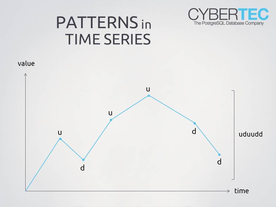
After this basic introduction, it is time to focus on the real trick. The idea is to use the output of the previous SQL statement and analyze the differences from one row to the next. In case the value is higher than zero, we encode it as “u” (for “up”) and in case it is not we use “d” (“down”). Where does this get us? Well, the advantage is that every move of the series is represented as a single character, which makes it easy to process later on. After the encoding process we use a sliding window. We take all the data from 5 periods (2 before, the current period and 2 later) and turn it into a single string.

The result is as follows:

test=# SELECT  *,
	string_agg(CASE WHEN diff > 0
			THEN 'u'::text
			ELSE 'd'::text END, '')
                OVER (ORDER BY id ROWS BETWEEN 2 PRECEDING
			AND 2 FOLLOWING) AS encoded
FROM    (   
                SELECT  *, data - lag(data, 1)
			OVER (ORDER BY id)  AS diff 
                FROM    
t_timeseries  
                ) AS x;
 id | data | diff | encoded
----+------+------+---------
  1 |   11 |      | duu
  2 |   14 |    3 | duud
  3 |   16 |    2 | duudu
  4 |    9 |   -7 | uuduu
  5 |   12 |    3 | uduuu
  6 |   13 |    1 | duuud
  7 |   14 |    1 | uuudu
  8 |    9 |   -5 | uudud
  9 |   15 |    6 | udud
 10 |    9 |   -6 | dud
(10 rows)

The encoded string starts with just three characters. The reason is that there are no preceding values, so we only see what is ahead of us in the future. The query gives us some data along with an encoded string.

The output of the query can be turned into a view:

CREATE VIEW v AS
SELECT  *, string_agg(CASE WHEN diff > 0
				THEN 'u'::text
				ELSE 'd'::text END, '')
                OVER (ORDER BY id ROWS BETWEEN 2 PRECEDING
				AND 2 FOLLOWING) AS encoded
FROM    (
        SELECT  *, data - lag(data, 1) OVER (ORDER BY id)  AS diff
        FROM    t_timeseries
) AS x;

Keep It Simple

Remember that this encoder is pretty simple and is usually not sufficient to process a real-world example. If you are planning to do real-world timeseries analysis in PostgreSQL, the encoder (“time series codec”) may be a better bet: it’s a lot more sophisticated. The point here is just to give you some ideas of what can be done with a fairly simple technique using a standard PostgreSQL database.

Analyzing an encoded string

Now that the data has been encoded it can be easily analyzed using standard PostgreSQL features. Suppose we want to find all parts of the data in which the value moved up at least 3 times in a row. The following query can be used:

test=# SELECT  * 
FROM    v 
WHERE   encoded LIKE '%uuu%';
 id | data | diff | encoded
----+------+------+---------
  5 |   12 |    3 | uduuu
  6 |   13 |    1 | duuud
  7 |   14 |    1 | uuudu
(3 rows)

Further tips for more complex patterns

You’ll want to use a more sophisticated search algorithm to find a more complex pattern than this. Regular expressions are a good tip and can be pretty useful in order to do that. It might also make sense to create a “distance” function and use KNN to look for areas in your timeseries which are similar to what you are looking for. Many analyses can be done if you are prepared to be a little creative.

Finally…

For more PG tips and tricks, find out how to speed up count(*) in PostgreSQL.

In order to receive regular updates on important changes in PostgreSQL, subscribe to our newsletter, or follow us on Twitter, Facebook, or LinkedIn.