How to interpret PostgreSQL EXPLAIN ANALYZE output

 

UPDATED July 2023: EXPLAIN ANALYZE is the key to optimizing SQL statements in PostgreSQL. This article does not attempt to explain everything there is to it. Rather, I want to give you a brief introduction, explain what to look for and show you some helpful tools to visualize the output.

Also, I want to call your attention to a new patch I wrote which has been included in PostgreSQL 16, EXPLAIN GENERIC PLAN. You can read about it here.

How to call EXPLAIN ANALYZE?

If you have an SQL statement that executes too slowly, you want to know what is going on and how to fix it. In SQL, it is harder to see how the engine spends its time, because it is not a procedural language, but a declarative language: you describe the result you want to get, not how to calculate it. The EXPLAIN command shows you the execution plan that is generated by the optimizer. This is helpful, but typically you need more information.

You can obtain such additional information by adding EXPLAIN options in parentheses.

The most important EXPLAIN options

• ANALYZE: with this keyword, EXPLAIN does not only show the plan and PostgreSQL's estimates, but it also executes the query (so be careful with UPDATE and DELETE!) and shows the actual execution time and row count for each step. This is indispensable for analyzing SQL performance.
• BUFFERS: You can only use this keyword together with ANALYZE, and it shows how many 8kB-blocks each step reads, writes and dirties. You always want this.
• VERBOSE: if you specify this option, EXPLAIN shows all the output expressions for each step in an execution plan. This is usually just clutter, and you are better off without it, but it can be useful if the executor spends its time in a frequently-executed, expensive function.
• SETTINGS: this option exists since v12 and includes all performance-relevant parameters that are different from their default value in the output.
• WAL: introduced in v13, this option shows the WAL usage incurred by data modifying statements. You can only use it together with ANALYZE. This is always useful information!
• FORMAT: this specifies the output format. The default format TEXT is the best for humans to read, so use that to analyze query performance. The other formats (XML, JSON and YAML are better for automated processing.

Typically, the best way to call EXPLAIN is:

Include SETTINGS if you are on v12 or better and WAL for data modifying statements from v13 on.

It is highly commendable to set track_io_timing = on to get data about the I/O performance.

Caveats and limitations

You cannot use EXPLAIN for all kinds of statements: it only supports SELECT, INSERT, UPDATE, DELETE, EXECUTE (of a prepared statement), CREATE TABLE ... AS and DECLARE (of a cursor).

Note that EXPLAIN ANALYZE adds a noticeable overhead to the query execution time, so don't worry if the statement takes longer.

There is always a certain variation in query execution time, as data may not be in cache during the first execution. That's why it is valuable to repeat EXPLAIN ANALYZE a couple of times and see if the result changes.

What information do you get from EXPLAIN ANALYZE?

PostgreSQL displays some of the information for each node of the execution plan, and you see some of it in the footer.

EXPLAIN without options

Plain EXPLAIN will give you the estimated cost, the estimated number of rows and the estimated size of the average result row. The unit for the estimated query cost is artificial (1 is the cost for reading an 8kB page during a sequential scan). There are two cost values: the startup cost (cost to return the first row) and the total cost (cost to return all rows).

Output from the ANALYZE option

ANALYZE gives you a second parenthesis with the actual execution time in milliseconds, the actual row count and a loop count that shows how often that node was executed. It also shows the number of rows that filters have removed.

In the footer, you see how long PostgreSQL took to plan and execute the query. You can suppress that information with SUMMARY OFF.

Output from the BUFFERS option

This option shows how many data blocks were found in the cache (hit) for each node, how many had to be read from disk, how many were written and how many dirtied. In recent versions, the footer contains the same information for the work done by the optimizer, if it didn't find all its data in the cache.

If track_io_timing = on, you will get timing information for all I/O operations.

How to read EXPLAIN ANALYZE output

You see that you end up with quite a bit of information even for simple queries. To extract meaningful information, you have to know how to read it.

First, you have to understand that a PostgreSQL execution plan is a tree structure consisting of several nodes. The top node (the Aggregate above) is at the top, and lower nodes are indented and start with an arrow (->). Nodes with the same indentation are on the same level (for example, the two relations combined with a join).

PostgreSQL executes a plan top down, that is, it starts with producing the first result row for the top node. The executor processes lower nodes “on demand”, that is, it fetches only as many result rows from them as it needs to calculate the next result of the upper node. This influences how you have to read “cost” and “time”: the startup time for the upper node is at least as high as the startup time of the lower nodes, and the same holds for the total time. If you want to find the net time spent in a node, you have to subtract the time spent in the lower nodes. Parallel queries make that even more complicated.

On top of that, you have to multiply the cost and the time with the number of “loops” to get the total time spent in a node.

What to focus on in EXPLAIN ANALYZE output

• Find the nodes where most of the execution time was spent.
• Find the lowest node where the estimated row count is significantly different from the actual row count. Very often, this is the cause of bad performance, and the long execution time somewhere else is only a consequence of a bad plan choice based on a bad estimate. “Significantly different” typically means a factor of 10 or so.
• Find long running sequential scans with a filter condition that removes many rows. These are good candidates for an index.

Tools to interpret EXPLAIN ANALYZE output

Since reading a longer execution plan is quite cumbersome, there are a few tools that attempt to visualize this “sea of text”:

Depesz' EXPLAIN ANALYZE visualizer

This tool can be found at https://explain.depesz.com/. If you paste the execution plan in the text area and hit “Submit”, you will get output like this:

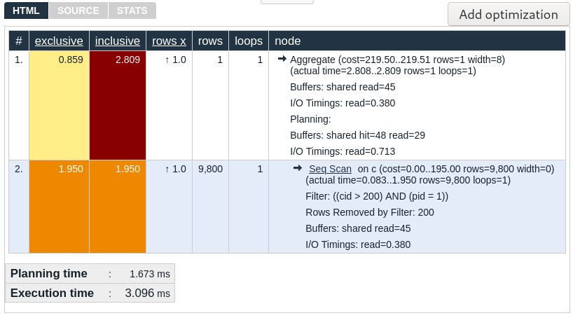
The execution plan looks somewhat similar to the original, but optically more pleasing. There are useful additional features:

• Total execution time and net execution time are calculated and shown for each node. This saves you a lot of work! The nodes with the highest times are highlighted with a red background and are easy to spot.
• Under the heading “rows x” you see by what factor PostgreSQL overestimated or underestimated the row count. Bad estimates are highlighted with a red background.
• If you click on a node, everything that is under it is hidden. That allows you to ignore uninteresting parts of a long execution plan and focus on the important ones.
• If you hover over a node, all its immediate children are highlighted with a star. That makes it easy to locate them in a big execution plan.

What I particularly like about this tool is that all the original EXPLAIN text is right there for you to see, once you have focused on an interesting node. The look and feel is decidedly more “old school” and no-nonsense, and this site has been around for a long time.

Dalibo's EXPLAIN ANALYZE visualizer

This tool can be found at https://explain.dalibo.com/. Again, you paste the raw execution plan and hit “Submit”. The output is presented as a tree:

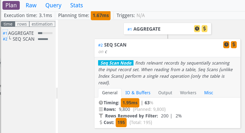
Initially, the display hides the details, but you can show them by clicking on a node, like I have done with the second node in the image above. On the left, you see a small overview over all nodes, and from there you can jump to the right side to get details. Features that add value are:

• On the left side, you see bars that represent the relative net execution time and allow you to focus on the most expensive nodes.
• Also on the left side, you can select “estimation” to see by how much PostgreSQL over- or underestimated the row count for each row.
• Finally, you can click on “buffers” to see which nodes used the most 8kB blocks. This is useful information, as it shows nodes whose execution time will depend on how well the data are cached.
• On the right side, you can expand a node by clicking on it, and get all the detailed information in several tabs.
• You can collapse everything underneath a node in the tree by clicking on the “crosshair” icon hidden in the lower right corner of a node.

The nice thing about this tool is that it makes the tree structure of the execution plan clearly visible. The look and feel is more up-to-date. On the downside, it hides the detailed information somewhat, and you have to learn where to search for it.

Conclusion

EXPLAIN (ANALYZE, BUFFERS) (with track_io_timing turned on) will show you everything you need to know to diagnose SQL statement performance problems. To keep from drowning in a sea of text, you can use Depesz' or Dalibo's visualizer. Both provide roughly the same features.

For more information on detailed query performance analysis, see my blog about using EXPLAIN(ANALYZE) with parameterized statements.

Before you can start tuning queries, you have to find the ones that use most of your server's resources. Here is an article that describes how you can use pg_stat_statements to do just that.

---

In order to receive regular updates on important changes in PostgreSQL, subscribe to our newsletter, or follow us on Twitter, Facebook, or LinkedIn.