written by Granthana Biswas

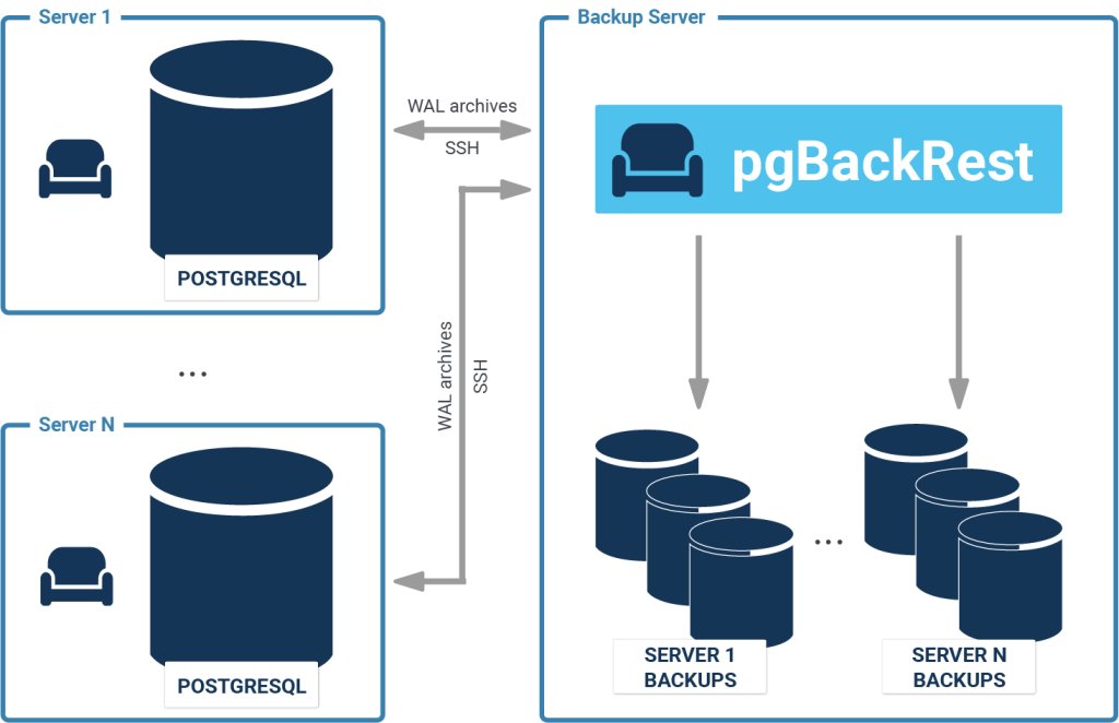
pgBackRest is an open source backup tool for PostgreSQL which offers easy configuration and reliable backups. So if you want to protect your database and create backups easily, pgBackRest is a good solution to make that happen. In this blog, we are going to go through the basic steps of using pgBackRest for full and differential backup of PostgreSQL.

Some of the key features of pgBackRest are:

1. Parallel backup & restore
2. Local and remote operations
3. Full, incremental & differential backups
4. Backup rotation & archive expiration
5. Backup integrity
6. Page checksums
7. Resume backups
8. Streaming compression and checksums

To read about them more in detail, please visit pgbackrest.org.

Here, we are going to build pgBackRest from the source and install it on the host where a test DB cluster is running.

Installation

Installing from Debian / Ubuntu packages:

For manual installation, download the source on a build host. Please avoid building the source on a production server, as the tools required should not be installed on a production machine:

Download pgBackRest Version 2.14:

Install the dependencies and check for 64-bit integers:

Build pgbackrest package:

Copy from build host to DB host:

Install Perl packages:

pgBackRest config files & directories on DB test host:

Create repository for pgBackRest

Set the Repo path and PostgreSQL cluster directory in the pgbackrest file:

[demo]

pg1-path=/data/postgres/pgdata/data1

[global]

repo1-path=/var/lib/pgbackrest

Configure archiving on the PostgreSQL cluster:

Change the following parameters in postgresql.conf:

Create stanza as postgres user:

The stanza-create command must be run on the host where the repository is located to initialize the stanza. It is recommended that the check command be run after stanza-create to ensure archiving and backups are properly configured.

Use the info command to get information about the backup

Since we haven't made any backups yet, we will get the following result:

Backup:

Let's make the first backup. By default, it will be full even if we specify type as differential:

Now when we run the info command again:

Take a differential backup of the cluster

To see the changes, check info:

If you want to learn more about how to protect data, check out my blog on PostgreSQL TDE ("Transparent Data Encryption") .

Also if you want to make sure that your database performs well, check out our blog posts on PostgreSQL performance.

Row Level Security (RLS) is one of the key features in PostgreSQL. It can be used to dramatically improve security and help to protect data in all cases. However, there are a couple of corner cases which most people are not aware of. So if you are running PostgreSQL and you happen to use RLS in a high-security environment, this might be the most important piece of text about database security you have ever read.

Row-Level-Security in PostgreSQL: Corner cases

To prepare for my examples let me create some data first. The following code is executed as superuser:

For the sake of simplicity there are only three users: postgres, bob, and alice. The t_service table contains six different services. Some are related to PostgreSQL and some to Oracle. The goal is to ensure that bob is only allowed to see Open Source stuff while alice is mostly an Oracle girl.

While hacking up the example, we want to see who we are and which chunks of code are executed as which user at all times. Therefore I have written a debug function which just throws out a message and returns true:

Now that the infrastructure is in place, RLS can be enabled for this table:

The superuser is not able to see all the data. Normal users are not allowed to see anything. To them, the table will appear to be empty.

Using CREATE POLICY in PostgreSQL

Of course, people want to see data. In order to expose data to people, policies have to be created. In my example there will be two policies:

What we see here is that bob is really the Open Source guy while alice is more on the Oracle side. I added the debug_me function to the policy so that you can see which users are active.

Let us set the current role to bob and run a simple SELECT statement:

The policy does exactly what you would expect for bob. The same thing is true for alice:

PostgreSQL Row-Level-Security and views

As a PostgreSQL consultant and PostgreSQL support company there is one specific question which keeps coming to us again and again: What happens if RLS (Row Level Security) is used in combination with views? This kind of question is not as easy to answer as some people might think. Expect some corner cases which require a little bit of thinking to get stuff right.

To show how things work, I will switch back to user “postgres” and create two identical views:

SELECT permissions will be granted to both views, but there is one more difference: alice will be the owner of v2. v1 is owned by the postgres user. This tiny difference makes a major difference later on, as you will see. To sum it up: v1 will be owned by postgres, v2 is owned by our commercial database lady alice, and everybody is allowed to read those views.

Let us see what happens:

Ooops! What is going on here? “bob” is allowed to see all the data. There is a reason for that: The view is owned by “postgres”. That means that the row level policy on t_service will not be taken into account. The RLS policies (Row Level Security) have been defined for bob and alice. However, in this case they are not taken into consideration, because the view is owned by the superuser, and the superuser has given us SELECT permissions on this view so we can see all that data. That is important: Imagine some sort of aggregation (e.g. SELECT sum(turnover) FROM sales). A user might see the aggregate but not the raw data. In that case, skipping the policy is perfectly fine.

The situation is quite different in the case of v2:

The “current_user” is still “bob” BUT what we see is only closed source data, which basically belongs to alice. Why does that happen? The reason is: v2 belongs to alice and therefore PostgreSQL will check alice's RLS policy. Remember, she is supposed to see closed source data and as the “owner” of the data she is in charge. The result is: bob will see closed source data, but no open source data (which happens to be his domain). Keep these corner cases in mind - not being aware of this behavior can create nasty security problems. Always ask yourself which policy PostgreSQL will actually use behind the scenes. Having a small test case at hand can be really useful in this context.

Solving the more common security challenges

What you have seen are some corner cases many people are not aware of. Our PostgreSQL consultants have seen some horrible mistakes in this area already, and we would like to ensure that other people out there don't make the same mistakes.

Let us drop those policies:

Usually policies are not assigned to individual people, but to a group of people or sometimes even to “public” (basically everybody who does not happen to be a superuser in this context). The following code snippet shows a simple example:

If the CURRENT_USER is bob, the system is supposed to show Open Source data. Otherwise it is all about closed source.

Let us take a look what happens:

The most important observation is that the policy applies to everybody who is not marked as superuser and it applies to everybody who is not marked with BYPASSRLS. As expected, alice will only see her subset of data:

The most important observation here is that defining policies has to be done with great care. ALWAYS make sure that your setup is well tested and that no leaks can happen. Security is one of the most important topics in any modern IT system and nobody wants to take chances in this area.

CYBERTEC can help to secure databases

As a PostgreSQL consulting company we can help to make sure that your databases are indeed secure. Leaks must not happen and we can help to achieve that.
If you want to learn more about PostgreSQL security in general, check out our PostgreSQL products including Data Masking for PostgreSQL which helps you to obfuscate data, and check out PL/pgSQL_sec which has been designed explicitly to protect your code.

---

In order to receive regular updates on important changes in PostgreSQL, subscribe to our newsletter, or follow us on Facebook or LinkedIn.

UPDATED July 2023: Window functions and analytics have been around for quite some time and many people already make use of this awesome stuff in the PostgreSQL world. Timeseries are an especially important area in this context. However, not all features have been widely adopted and thus many developers have to implement functionality at the application level in a painful way instead of just using some of the more advanced SQL techniques.

The idea of this blog is to demonstrate some of the advanced analytics so that more people out there can make use of PostgreSQL's true power.

Preparing data for analytics

For the purpose of this post I have created a basic data set:

Useful functions

In PostgreSQL, the generate_series function will return one row each day spanning January 2nd, 2020 to January 15th, 2020. The WITH ORDINALITY clause tells PostgreSQL to add an “id” column to the result set of the function. The date_part function will extract the number of the week out of our date. The purpose of this column is to have a couple of identical values in our timeseries.

In the next list you see the data set we'll use:

Sliding windows: Moving over timeseries in SQL

One of the things you often have to do is to use a sliding window. In SQL this can easily be achieved using the OVER clause. Here is an example:

OVER and array_agg

The OVER clause allows you to feed the data to the aggregate function. For the sake of simplicity, I have used the array_agg function, which simply returns the data fed to the aggregate as an array. In a real-life scenario you would use something more common such as the avg, sum, min, max, or any other aggregation function. However, array_agg is pretty useful, in that it shows which data is really passed to the function, and what values we have in use. ROWS BETWEEN … PRECEDING AND 1 … FOLLOWING tells the system that we want to use 3 rows: The previous, the current one, as well as the one after the current row. At the beginning of the list, there is no previous row, so we will only see two values in the array column. At the end of the data set, there are also only two rows, because there are no more values after the last one.

The EXCLUDE CURRENT ROW clause

In some cases, it can be useful to exclude the current row from the data passed to the aggregate. The EXCLUDE CURRENT ROW clause has been developed to do exactly that. Here is an example:

As you can see, the array is a little shorter now. The current value is not part of the array anymore.

Timeseries with SQL: Making use of EXCLUDE TIES

The idea behind EXCLUDE TIES is to remove duplicates. Let's take a look at the following to make things clear:

EXCLUDE TIES: Explanation

The first array_agg simply collects all values in the frame we have defined. The “ties” column is a bit more complicated to understand: Let's take a look at the 5th of January. The result says (1, 2, 2). As you can see, two incarnations of 1 have been removed. EXCLUDE TIES made sure that those duplicates are gone. However, this has no impact on those values in the “future”, because the future values are different from the current row. The documentation states what EXCLUDE TIES is all about: “EXCLUDE TIES excludes any peers of the current row from the frame, but not the current row itself.”

After this first example, we should also consider a fairly common mistake:

Spot the difference - find the mistake

Can you spot the difference between this and the previous example? Take all the time you need …
The problem is that the ORDER BY clause has two columns in this case. That means that there are no duplicates anymore from the ORDER BY's perspective. Thus, PostgreSQL is not going to prune values from the result set. I can assure you that this is a common mistake seen in many cases. The problem can be very subtle and go unnoticed for quite some time.

Excluding entire groups from a window function

In some cases you might want to remove an entire set of rows from the result set. To do that, you can make use of EXCLUDE GROUP.

The following example shows how that works, and how our timeseries data can be analyzed:

Understanding the results

The first aggregation function does ORDER BY week and the array_agg will aggregate on the very same column. In this case, we will see a couple of NULL columns, because in some cases all entries within the frame are simply identical. The last row in the result set is a good example: All array entries are 3 and the current row contains 3 as well. Thus all incarnations of 3 are simply removed, which leaves us with an empty array.

To calculate the last column, the data is ordered by day. In this case, there are no duplicates and therefore no data can be removed. For more information on EXCLUDE GROUP, see the documentation on window functions.

DISTINCT: Dealing with duplicates from timeseries data

In PostgreSQL, an aggregate function is capable of handling DISTINCT. The following example shows what I mean:

What does count do?

“count” does not simply count all columns, but filters the duplicates beforehand. Therefore the result is simply 3.
In PostgreSQL there is no way to use DISTINCT as part of a window function. PostgreSQL will simply error out:

Avoiding DISTINCT

The natural question which arises is: How can we achieve the same result without using DISTINCT inside the window function? What you have to do is to filter the duplicates on a higher level. You can use a subselect, unroll the array, remove the duplicates and assemble the array again. It is not hard to do, but it is not as elegant as one might expect.

Further reading

In case you are interested in timeseries and aggregation in general, consider checking out some of our other blog posts including “Speeding up count(*)” by Laurenz Albe. If you are interested in high-performance PostgreSQL check out my blog post about finding slow queries.

---

In order to receive regular updates on important changes in PostgreSQL, subscribe to our newsletter, or follow us on Facebook or LinkedIn.

Trivial timeseries are an increasingly important topic - not just in PostgreSQL. Recently I gave a presentation @AGIT in Salzburg about timeseries and I demonstrated some super simple examples. The presentation was well received, so I decided to share this stuff in the form of a blog, so that more people can learn about window functions and SQL in general. A link to the video is available at the end of the post so that you can listen to the original material in German.

Loading trivial timeseries data the easy way

To show how data can be loaded, I compiled a basic dataset which can be found on my website. Here is how it works:

The cool thing is that if you happen to be a superuser, you can easily load the data from the web directly. COPY FROM PROGRAM allows you to execute code on the server and pipe it directly to PostgreSQL, which is super simple. Keep in mind: that only works if you are a PostgreSQL superuser (for security reasons).

lag: The backbone of trivial timeseries analysis

If you are dealing with timeseries, calculating the difference to the previous period is really important. Fortunately, SQL allows you to do that pretty easily. Here is how it works:

The lag functions takes two parameters: The first column defines the column, which should be used in this case. The second parameter is optional. If you skip it, the expression will be equivalent to lag(production, 1). In my example, the lag column will be off by one. However, you can use any integer number to move data up or down, given the order defined in the OVER clause.

What we have so far is the value of the previous period. Let us calculate the difference next:

That was easy. All we have to do is to take the current row and subtract the previous row.
Window functions are far more powerful than shown here, but maybe this example will help to get you started in the first place.

Calculating correlations using PostgreSQL

You may want to calculate the correlation between columns. PostgreSQL offers the “corr” function to do exactly that. The following listing shows a simple example:

As you can see, the correlation in Mexico and Canada are highest.

Checking for continuous activity

In the past we presented other examples related to timeseries and analysis in general. One of the most interesting posts is found here.

If you want to see the entire short presentation in German consider checking out the following video.

---

In order to receive regular updates on important changes in PostgreSQL, subscribe to our newsletter, or follow us on Facebook or LinkedIn.