I have already written about timeseries and PostgreSQL in the past. However, recently I stumbled across an interesting problem, which caught my attention: Sometimes you might want to find “periods” of activity in a timeseries. For example: When was a user active? Or when did we receive data? This blog post tries to give you some ideas and shows, how you can actually approach this kind of problem.
Table of Contents
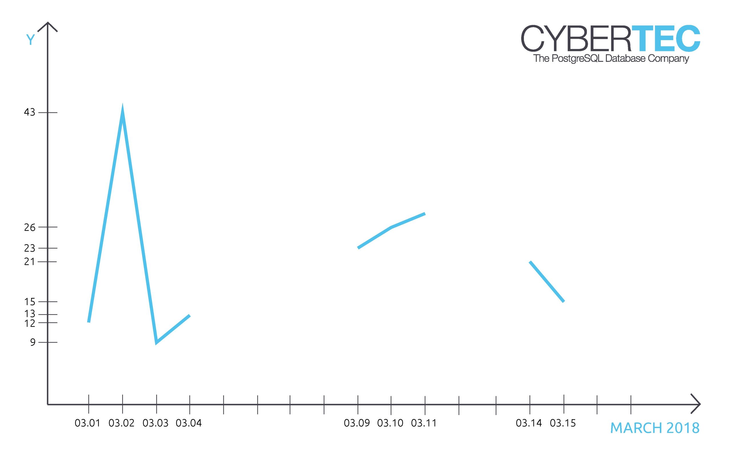
The next listing shows a little bit of sample data, which I used to write the SQL code you are about to see:
|
1 2 3 4 5 6 7 8 9 10 11 12 13 |
CREATE TABLE t_series (t date, data int); COPY t_series FROM stdin DELIMITER ';'; 2018-03-01;12 2018-03-02;43 2018-03-03;9 2018-03-04;13 2018-03-09;23 2018-03-10;26 2018-03-11;28 2018-03-14;21 2018-03-15;15 . |
To make it easier, I just used two columns in my example. Note that my timeseries is not continuous but interrupted. There are three continuous periods in this set of data. Our goal is to find and isolate them to do analysis on each of those continuous periods.
When dealing with timeseries, one of the most important things to learn is how to “look forward and backward”. In most cases, it is simply vital to compare the current line with the previous line. To do that in PostgreSQL (or in SQL in general) you can make use of the “lag” function:
|
1 2 3 4 5 6 7 8 9 10 11 12 13 14 |
test=# SELECT *, lag(t, 1) OVER (ORDER BY t) FROM t_series; t | data | lag ------------+------+---------- 2018-03-01 | 12 | 2018-03-02 | 43 | 2018-03-01 2018-03-03 | 9 | 2018-03-02 2018-03-04 | 13 | 2018-03-03 2018-03-09 | 23 | 2018-03-04 2018-03-10 | 26 | 2018-03-09 2018-03-11 | 28 | 2018-03-10 2018-03-14 | 21 | 2018-03-11 2018-03-15 | 15 | 2018-03-14 (9 rows) |
As you can see, the last column contains the date of the previous row. Now: How does PostgreSQL know what the previous row actually is? The “ORDER BY”-clause will define exactly that.
Based on this query you have just seen it will be easy to calculate the size of the gap from one row to the next row
|
1 2 3 4 5 6 7 8 9 10 11 12 13 14 |
test=# SELECT *, t - lag(t, 1) OVER (ORDER BY t) AS diff FROM t_series; t | data | diff ------------+------+------ 2018-03-01 | 12 | 2018-03-02 | 43 | 1 2018-03-03 | 9 | 1 2018-03-04 | 13 | 1 2018-03-09 | 23 | 5 2018-03-10 | 26 | 1 2018-03-11 | 28 | 1 2018-03-14 | 21 | 3 2018-03-15 | 15 | 1 (9 rows) |
What we see now is the difference from one period to the next. That is pretty useful because we can start to create our rules. When do we consider a segment to be over and how long of a gap to we allow for before we consider it to be the next segment / period?
In my example I decided that every gap, which is longer than 2 days should trigger the creation of a new segment (or period): The next challenge is therefore to assign numbers to each period, which are about to detect. Once this is done, we can easily aggregate on the result. The way I have decided to do this is by using the sum function. Remember: When NULL is fed to an aggregate, the aggregate will ignore the input. Otherwise it will simply start to add up the input.
Here is the query:
|
1 2 3 4 5 6 7 8 9 10 11 12 13 14 15 16 17 |
test=# SELECT *, sum(CASE WHEN diff IS NULL OR diff <2 THEN 1 ELSE NULL END) OVER (ORDER BY t) AS period FROM (SELECT *, t - lag(t, 1) OVER (ORDER BY t) AS diff FROM t_series ) AS x; t | data | diff | period ------------+------+------+-------- 2018-03-01 | 12 | | 1 2018-03-02 | 43 | 1 | 1 2018-03-03 | 9 | 1 | 1 2018-03-04 | 13 | 1 | 1 2018-03-09 | 23 | 5 | 2 2018-03-10 | 26 | 1 | 2 2018-03-11 | 28 | 1 | 2 2018-03-14 | 21 | 3 | 3 2018-03-15 | 15 | 1 | 3 (9 rows) |
As you can see the last column contains the period ID as generated by the sum function in our query. From now on analysis will be pretty simple as we can simply aggregate over this result using a simple subselect as shown in the next statement:
|
1 2 3 4 5 6 7 8 9 10 11 12 13 14 15 |
test=# SELECT period, sum(data) FROM (SELECT *, sum(CASE WHEN diff IS NULL OR diff <2 THEN 1 ELSE NULL END) OVER (ORDER BY t) AS period FROM (SELECT *, t - lag(t, 1) OVER (ORDER BY t) AS diff FROM t_series ) AS x ) AS y GROUP BY period ORDER BY period; period | sum --------+----- 1 | 77 2 | 77 3 | 36 (3 rows) |
The result displays the sum of all data for each period. Of course you can also do more complicated stuff. However, the important thing is to understand, how you can actually detect various periods of continuous activity.
In order to receive regular updates on important changes in PostgreSQL, subscribe to our newsletter, or follow us on Facebook or LinkedIn.
Hi,
SELECT *, sum(CASE WHEN diff IS NULL
OR diff <2 THEN 1 ELSE NULL END) OVER (ORDER BY t) AS period
FROM (SELECT *, t - lag(t, 1) OVER (ORDER BY t) AS diff
FROM t_series
) AS x;
is generating seven periods
1 12
2 43
3 9
4 36
5 26
6 49
7 15
but if I have changed your query as follows, I am getting the correct results.
select period, sum(data) from
(select *, sum(case when diff is null or diff < 2 then 0 else 1 end) over (order by t) as period
from (select *, t - lag(t, 1) over (order by t) as diff from t_series) as x) as y
group by period
order by period;
0 77
1 77
2 36
which is the one should I use?
yeah, nice, but your example doesn't work 😉
with your data and sql:
test=*# SELECT *, sum(CASE WHEN diff IS NULL
test(# OR diff = 2 then 1 else NULL end) over (order by t),0) from (select *, t - coalesce(lag(t,1) over (order by t),t) as diff from t_series) foo ;
t | data | diff | ?column?
------------ ------ ------ ----------
2018-03-01 | 12 | 0 | 1
2018-03-02 | 43 | 1 | 1
2018-03-03 | 9 | 1 | 1
2018-03-04 | 13 | 1 | 1
2018-03-09 | 23 | 5 | 2
2018-03-10 | 26 | 1 | 2
2018-03-11 | 28 | 1 | 2
2018-03-14 | 21 | 3 | 3
2018-03-15 | 15 | 1 | 3
(9 Zeilen)
now i'm getting the expected result 😉 But anyway, nice article, thx.