By Kaarel Moppel - Some weeks ago, in the light of PostgreSQL v12 release, I wrote a general overview on various major version upgrade methods and benefits of upgrading in general - so if upgrading is a new thing for you I’d recommend to read that posting first. But this time I’m concentrating on the newest (available since v10) and the most complex upgrade method - called “Logical Replication” or LR shortly. For demonstration purposes I’ll be migrating from v10 to freshly released v12 as this is probably the most likely scenario. But it should work the same also with v11 to v12. But do read on for details.

Benefits of LR upgrades

First a bit of recap from the previous post on why would you use LR for upgrading at all. Well, in short - because it’s the safest option with shortest possible downtime! With that last point I’m already sold...but here again the list of “pros” / “cons”:

PROS

• Minimal downtime required

After the initial setup burden one just needs to wait (and verify) that the new instance hast all the data from the old one...and then just shut down the old instance and point applications to the new instance. Couldn’t be easier!

Also before the switchover one can make sure that statistics are up to date, to minimize the typical “degraded performance” period seen after "pg_upgrade" for more complex queries (on bigger databases). For high load application one could even be more careful here and pull the most popular relations into shared buffers by using the (relatively unknown) “pg_prewarm” Contrib extension or by just running common SELECT-s in a loop, to counter the “cold cache” effect.

• Flexible

One can for example already make some changes on the target DB – add columns / indexes, change datatypes, leave out some old archive tables, etc. The general idea is that LR does not work on the binary, 1-to-1 level as”pg_upgrade” does, but rather JSON-like data objects are sent over to another master / primary instance, providing quite some freedom on the details.

• Safe

Before the final switchover you can anytime abort the process and re-try if something seems fishy. The old instances data is not changed in any way even after the final switchover! Meaning you can easily roll back (with cost of some data loss typically though) to the old version if some unforeseen issues arise. One should only watch out for the replication slot on the source / publisher DB if the target server just taken down suddenly.

CONS

• Quite a few steps to take and possibly one needs to modify the schema a bit.
• Always per DB.
• Could take a long time for big databases.
• Large objects, if in use (should be a thing of the past really), need to be exported / imported manually.

Preparing for LR

As LR has some prerequisites on the configuration and schema, you’d first need to see if it’s possible to start with the migration process at all or some changes are needed on the old master node, also called the “publisher” in LR context.

Action points:

1) Enable LR on the old master aka subscriber aka source DB if not done already. This means setting “wal_level” to “logical” in postgresql.conf and making sure that “replication” connections are allowed in “pg_hba.conf” from the new host (also called the “subscriber” in LR context). FYI - changing “wal_level” needs server restart! To enable any kind of streaming replication some other params are needed but they are actually already set accordingly out of the box as of v10 so it shouldn’t be a problem.

2) Check that all tables have a Primary Key (which is good database design anyways) or alternatively have REPLICA IDENTITY set. Primary Keys don’t need much explaining probably but what is this REPLICA IDENTITY thing? A bit simplified - basically it allows to say which columns formulate uniqueness within a table and PK-s are automatically counted as such.

3) If there’s no PK for a particular table, you should create one, if possible. If you can’t do that, set unique constraints / indexes to serve as REPLICA IDENTITY, if at all possible. If even that isn’t possible, you can set the whole row as REPLICA IDENTITY, a.k.a. REPLICA IDENTITY FULL, meaning all columns serve as PK’s in an LR context - with the price of very slow updates / deletes on the subscriber (new DB) side, meaning the whole process could take days or not even catch up, ever! It’s OK not to define a PK for a table, as long as it’s a write-only logging table that only gets inserts.

Sample code:

Fresh setup of the new “subscriber” DB

Second most important step is to set up a new totally independent instance with a newer Postgres version - or at least create a new database on an existing instance with the latest major version. And as a side note - same version LR migrations are also possible, but you'd be solving some other problem in that case.

This step is actually very simple - just a standard install of PostgreSQL, no special steps needed! With the important addition that to make sure everything works exactly the same way as before for applications - same encoding and collation should be used!

NB! Before the final switchover it’s important that no normal users have access to the new DB - as they might alter table data or structures and thereby inadvertently produce replication conflicts that mostly mean starting from scratch (or a costly investigation / fix) as “replay” is a sequential process.

Schema / roles synchronization

Next we need to synchronize the old schema onto the new DB as Postgres does not take care of that automatically as of yet. The simplest way is to use the official PostgreSQL backup tool called “pg_dump”, but if you have your schema initialization scripts in Git or such and they're up to date then this is fine also. For syncing roles “pg_dumpall” can be used.

NB! After this point it’s not recommended to introduce any changes to the schema or be at least very careful when doing it, e.g. creating new tables / columns first on the subscriber and refreshing the subscriptions when introducing new tables - otherwise data synchronization will break! Tip - a good way to disable unwanted schema changes is to use DDL triggers! An approximate example on that is here. Adding new tables only on the new DB is no issue though but during an upgrade not a good idea anyways - my recommendation is to first upgrade and then to evolve the schema.

Create a “publication” on the old DB

If preparations on the old DB has been finished (all tables having PK-s or replication identities) then this is a oneliner:

Here we added all (current and those added in future) tables to a publication (a replication set) named “upgrade” but technically we could also leave out some or choose to only replicate some operations like UPDATE-s, but for a pure version upgrade you want typically all.

NB! As of this moment the replication identities become important - and you might run into trouble on the old master if the identities are not in place on all tables that get changes! In such case you might see errors like that:

Create a “subscription” on the target DB

Next step - create a “subscription” on the new DB. This is also a oneliner, that creates a logical replication slot on the old instance, pulls initial table snapshots and then starts to stream and apply all table changes as they happen on the source, resulting eventually in a mirrored dataset! Note that currently superuser rights are needed for creating the subscription and actually hit also makes life a lot easier on the publisher side.

WARNING! As of this step the 2 DB-s are “coupled” via a replication slot, carrying some dangers if the process is aborted abruptly and the old DB is not “notified” of that. If this sounds new please see the details from documentation.

Check replication progress

Depending on the amount of data it will take X minutes / days until everything is moved over and “live” synchronization is working.

Things to inspect for making sure there are no issues:

• No errors in server logs on both sides
• There’s an active “pg_replication_slots” entry on the master with the name that we used to create the “subscription” on the new DB
• All tables are actively replicating on the subscriber side, i.e. “pg_subscription_rel.srsubstate” should be ‘r’ for all tables (ready - normal replication)

Basic data verification / switchover preparation

Although not a mandatory step, when it comes to data consistency / correctness, it always makes sense to go the extra mile and run some queries that validate that things (source - target) have the same data. For a running DB it’s of course a bit difficult as there’s always some replication lag but for “office hours” applications it should make a lot of sense. My sample script for comparing rowcounts (in a non-threaded way) is for example here but using some slightly more "costly" aggregation / hashing functions that really look at all the data would be even better there.

Also important to note if you’re using sequences (which you most probably are) - sequence state is not synchronized by LR and needs some manual work / scripting! The easiest option I think is that you leave the old DB ticking in read-only mode during switchover so that you can quickly access the last sequence values without touching the indexes for maximum ID-s on the subscriber side.

Switchover time!

We’re almost there with our little undertaking...with the sweaty part remaining - the actual switchover to start using the new DB! Needed steps are simple though and somewhat similar to switching over to a standard, “streaming replication” replica.

1) Re-check the system catalog views on replication status.

2) Stop the old instance.

Make sure it’s a nice shutdown. The last logline should state “database system is shut down”, meaning all recent changes were delivered to connected replication clients, including our new DB. Start of downtime! PS Another alternative to make sure absolutely all data is received is to actually configure the new instance in “synchronous replication” mode! This has the usual synchronous replication implications of course so I’d avoid it for bigger / busier DBs.

3) Start the old DB in read-only mode by creating a recovery.conf file

From v12 this is achieved by declaring a "standby.signal" file

4) Optionally make some more quick “health checks”

if time constraints allow it - verify table sizes, row counts, your last transactions, etc. For “live” comparisons it makes sense to restart the old DB under a new, random port so that no-one else connects to it.

5) Synchronize the sequences.

Given we'll leave the old DB in read-only mode the easiest way is something like that:

6) Reconfigure

your pg_hba.conf to allow access for all "mortal" users, then reconfigure your application, connection pooler, DNS or proxy to start using the new DB! If the two DB-s were on the same machine then it’s even easier - just change the ports and restart. End of downtime!

7) Finish

Basically we’re done here, but would be nice of course to clean up and remove the (no-more needed) subscription not to accumulate errors in server log.

Note that if you won't keep the old “publisher” accessible in read-only or normal primary mode (dangerous!) though, some extra steps are needed here before dropping:

8) Time for some bubbly drinks 🙂 

Summary

Although there are quite some steps and nuances involved, LR is worth adding to the standard upgrade toolbox for time-critical applications as it’s basically the best way to do major version upgrades nowadays - minimal dangers, minimal downtime!

FYI - if you're planning to migrate dozens of DB-s the LR upgrade process can be fully automated! Even starting from version 9.4 actually, with the help of the “pglogical” extension. So feel free to contact us if you might need something like that and don't particularly enjoy the details. Thanks for reading!

By Kevin Speyer

After reading this post you will be able to write your first Reinforcement Learning program to solve a real life problem - and beat Google at it.

Reinforcement Learning (RL) has gained a lot of attention due to its ability to surpass humans at numerous table games like chess, checkers and Go. If you are interested in AI, you have surely seen the video where a RL trained program finishes a Supermario level.

In this post, I'll show you how to write your first RL program from scratch. Then, I'll show how this algorithm manages to find better solutions for the Travelling Salesman Problem (TSP) than Google’s specialised algorithms. I will not go through the mathematical details of RL. You can read an introduction of Reinforcement Learning in this article and also in this article.

Q-learning

We will use a model-free RL named Q-learning. The key element in this algorithm is Q(s,a), which gives a score for each action (a) to take, given the state (s) that the agent is in. During training, the agent will go through various states and estimate what the total reward for each possible action is, taking into account the short- and long-term consequences. Mathematically speaking, this is written:

The parameters are alpha (learning rate) and gamma (discount factor). r(s,a) is the immediate reward for taking actions a under state s. The second term,  max_a' ( Q(a,a') ), is the tricky one. This adds the future reward to Q(s,a) so that long-term objectives are taken into account in Q(s,a). Gamma is a discount factor between 0 and 1 that gives a lower weight to distant events in the future.

Mapping the problem

Now it's just a matter of mapping states, rewards and actions to a specific problem. We will solve the Travelling Salesman Problem using Q-learning. Given a set of travelling distances between destinations, the problem is to find the shortest route to visit every location. In this case, we will start and finish in the same location, so it's a round trip. Now we need to map the problem to the algorithm.

Naturally, the state s is the location the salesman is at. The possible actions are the points he can visit; that was easy! Now, what is the immediate reward for going from point 0 to point 1? We want the reward to be a monotonic descendent function with respect to travelling distance. That is: less distance, more reward. In this case I used r(s,a) = 1/d_sa, where d_sa is the travelling distance between point s and point a. We are assuming that there is no 0 distance travel between points. Another possibility is to use r(s,a)=-d_sa.

Hands on: getting the data

First, we have to obtain the data. In this case, the given data is the location of each city to be visited by the salesman. Typically, this kind of data is stored in databases (DB). This means that we have to connect and query the DB to extract the relevant information. In this case I used PostgreSQL due to its features and simplicity. The programming language of choice for this project is python, because it is the most popular option for data science projects.

Let’s set the connection to the DB:

In usname and db_name you should write your username and database name, respectively. Now we have to query the DB, and get the position of each city:

Finally, we have to calculate the distances between each pair of cities and save it as a matrix:

Training the model

We will define just one function which will be responsible for updating the elements of the Q-matrix in the training phase according to equation 1.

Now we can train the RL model by letting the agent run through all the destinations, collecting the rewards. We will use 2000 training iterations.

The parameter epsilon (between 0 and 1) controls the exploration vs exploitation ratio in training. If epsilon is near 1, then the agent will take random decisions and explore new possibilities. A low value of epsilon means the agent will take the best known path, exploiting the information already acquired. A well-known policy is to lower this epsilon parameter as the model gains insight into the problem. At the beginning, the agent takes random actions and explores different routes, and as the Q matrix gains more useful information, the agent is more likely to take the path of greater reward.

Running the model

The agent starts at the warehouse and runs through all cities according to the Q matrix, trying to minimise the total distance of the route.

Example

To compare the solutions given by this algorithm, we will use the QR-tools TSP solver from Google. This is a highly specialised algorithm particularly designed to solve the TSP, and has great performance. After playing around with the RL algorithm and tuning the parameters (alpha and gamma), I was surprised to see that our RL algorithm was able to find shorter routes than Google's algorithm in some cases.

The Reinforcement Learning algorithm was able to beat the highly specific algorithm by almost 7%! It is worth mentioning that most of the time, OR-Tools’ algorithm finds the best solution, but not infrequently, our simple RL algorithm finds a better solution.

 

 

“Durability”, the D of ACID, demands that a committed database transaction remains committed, no matter what. For normal outages like a power failure, this is guaranteed by the transaction log (WAL). However, if we want to guarantee durability even in the face of more catastrophic outages that destroy the WAL, we need more advanced methods.

This article discusses how to use pg_receivewal to maintain durability even under dire circumstances.

Archiving WAL with archive_command

The “traditional” method of archiving the transaction log is the archive_command in postgresql.conf. The DBA has to set this parameter to a command that archives a WAL segment after it is completed.

Popular methods include:

• Use cp (or copy on Windows) to copy the file to network attached storage like NFS.
• Call a command like scp or rsync to copy the file to a remote machine.
• Call an executable from your favorite PostgreSQL backup software

The important thing to consider is that the archived WAL segment is stored somewhere else than the database.

I have a redundant distributed storage system, do I still need to store WAL archives somewhere else?

Yes, because there is still a single point of failure: the file system.
If the file system becomes corrupted through a hardware or software problem, all the redundant distributed copies of your WAL archive can vanish or get corrupted.

If you believe that this is so unlikely that it borders on the paranoid: I have seen it happen.
A certain level of professional paranoia is a virtue in a DBA.

When archive_command isn't good enough

If your database server gets destroyed so that its disks are no longer available, we will still lose some committed transactions: the transactions in the currently active WAL segment. Remember that PostgreSQL archives a WAL segment usually when it is full. So up to 16MB worth of committed transactions can vanish with the active WAL segment.

To reduce the impact, you can set archive_timeout: that will set the maximum time between WAL archivals. But for some applications, that just isn't good enough: If you cannot afford to lose a single transaction even in the event of a catastrophe, WAL archiving just won't do the trick.

pg_receivewal comes to the rescue

PostgreSQL 9.2 introduced pg_receivexlog, which has been renamed to pg_receivewal in v10. This client program will open a replication connection to PostgreSQL and stream WAL, just like streaming replication does. But instead of applying the information to a standby server, it writes it to disk. This way, it creates a copy of the WAL segments in real time. The partial WAL segment that pg_receivewal is currently writing has the extension .partial to distinguish it from completed WAL archives. Once the segment is complete, pg_receivewal will rename it.

pg_receivewal is an alternative to WAL archiving that avoids the gap between the current and the archived WAL location. It is a bit more complicated to manage and monitor, because it is a separate process and should run on a different machine.

pg_receivewal and synchronous replication

By default, replication is asynchronous, so pg_receivewal can still lose a split second's worth of committed transactions in the case of a crash. If you cannot even afford that, you can switch to synchronous replication. That guarantees that not a single committed transaction can get lost, but it comes at a price:

• Since every commit requires a round trip to pg_receivewal, it will take significantly longer. This has an impact on the number of writing transactions your system can support.
  Keep the network latency low!
• If you have only a single synchronous standby server (pg_receivewal acts as a standby), the availability of your system is reduced. This is because PostgreSQL won't commit any more transactions if your only standby is unavailable.
  To avoid that problem, you need at least two synchronous pg_receivewal processes.

Archive recovery and partial WAL segments

Now if the worst has happened and you need to recover, you'll have to make sure to restore the partial WAL segments as well. In the simple case where you archive to an NFS mount, the restore_command could be as simple as this:

Conclusion

With careful design and a little effort, you can set up a PostgreSQL system that can never lose a single committed transaction even under the most dire circumstances. Integrate this with a high availability setup for maximum data protection.

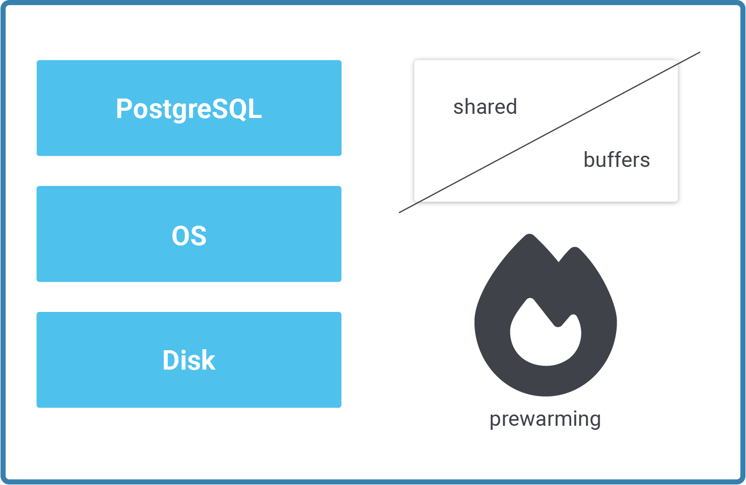
PostgreSQL uses shared_buffers to cache blocks in memory. The idea is to reduce
disk I/O and to speed up the database in the most efficient way
possible. During normal operations your database cache will be pretty useful and
ensure good response times. However, what happens if your database instance is
restarted - for whatever reason? Your PostgreSQL database performance will suffer
until your I/O caches have filled up again. This takes some time and it can
be pretty damaging to your query response times.

pg_prewarm: Filling up your database cache

Fortunately, there are ways in PostgreSQL to fix the problem. pg_prewarm is a
module which allows you to automatically prewarm your caches after a database
failure or a simple restart. The pg_prewarm module is part of the PostgreSQL
contrib package and is usually available on your server by default.
There is no need to install additional third party software. PostgreSQL has all
you need by default.

Warming caches manually or automatically.

Basically, pg_prewarm can be used in two ways:

• Manual caching
• Automatic caching on startup

Let us take a look at both options and see how the module works in detail. In general automatic pre-warming is, in my judgement, the better way to preload caches - but in some cases, it can also make sense to just warm caches manually (usually for testing purposes).

pg_prewarm: Putting data into shared_buffers manually

Prewarming the cache manually is pretty simple. The following section explains how the process works in general.

The first thing to do is to enable the pg_prewarm extension in your database:

To show how a table can be preloaded, I will first create a table and put it into
the cache:

All you have to do is to call the pg_prewarm function and pass the name of the
desired table to the function. In my example, 4425 pages have been read and put
into the cache.
4425 blocks translates to roughly 35 MB:

Calling pg_prewarm with one parameter is the easiest way to get started.
However, the module can do a lot more, as shown in the next listing:

In addition to passing the name of the object you want to cache to the function,
you can also tell PostgreSQL which part of the table you want to cache. The
"relation fork" defines whether you want the real data file, the VM (Visibility
Map) or the FSM (Free Space Map). Usually, caching the main table is just fine.
You can also tell PostgreSQL to cache individual blocks. While this is flexible,
it is usually not what you want to do manually.

Automatically populate your PostgreSQL I/O cache

In most cases, people might want pg_prewarm to take care of caching automatically
on startup. The way to achieve this is to add pg_prewarm to
shared_preload_libraries and to restart the database server. The following
example shows how to configure shared_preload_libraries in postgresql.conf:
shared_preload_libraries = 'pg_stat_statements, pg_prewarm'
After the server has restarted you should be able to see the "autoprewarm
master" process which is in charge of starting up things for you.

By default, pg_prewarm will store a list of blocks which are currently in memory
on disk. After a crash or a restart, pg_prewarm will automatically restore the
cache as it was when the file was last exported.

When to use pg_prewarm

In general, pg_prewarm makes most sense if your database and your RAM are really
really large (XXX GB or more). In such cases, the difference between cached
and uncached data will be greatest and users will suffer the most if
performance is bad.

Finally ...

If you want to learn more about performance and database tuning in general,
consider checking out my post about how to track down slow or time consuming
queries. You might also be interested in taking a look at
http://pgconfigurator.cybertec.at, which is a free website to help you with
database configuration.

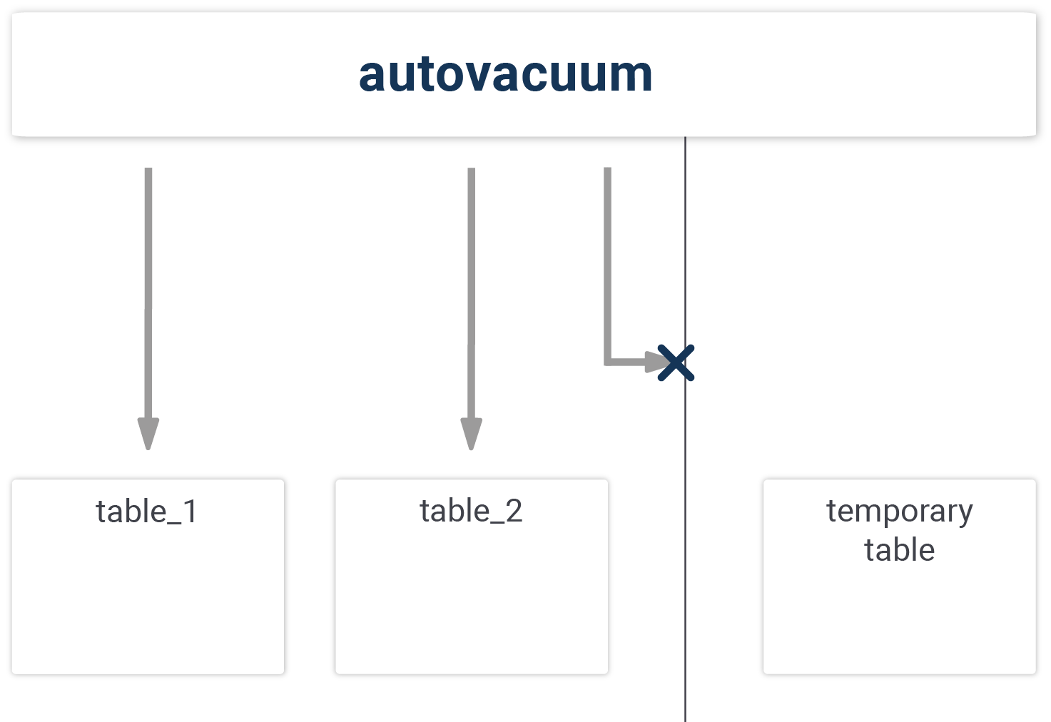
Did you know that your temporary tables are not cleaned up by autovacuum?

Autovacuum cleans tables automatically

Since the days of PostgreSQL 8.0, the database has provided the miraculous autovacuum daemon which is in charge of cleaning tables and indexes. In many cases, the default configuration is absolutely ok and people don’t have to worry about VACUUM much. However, recently one of our support clients sent us an interesting request related to temporary tables and autovacuum.

What is the problem?

The main issue is that autovacuum does not touch temporary tables. Yes, it’s true – you have to VACUUM temporary tables on your own. But why is this the case? Let’s take a look at how the autovacuum job works in general. Autovacuum sleeps for a minute and wakes up. After that it checks, if a table has seen a sufficiently large number of changes before it fires up a cleanup process. The important thing is that the cleanup process actually has to see the objects it will clean, and this is where the problem starts.

An autovacuum process has no way of seeing a temporary table, because temporary tables can only be seen by the database connection which actually created them. Autovacuum therefore has to skip temporary tables. Unfortunately, most people are not aware of this issue. As long as you don’t use your temporary tables for extended periods, the missing cleanup job is not an issue. However, if your temp tables are repeatedly changed in long transactions, it can become a problem.

Proving my point

The main question now is: How can we verify what I have just said? To show you what I mean, I will load the pgstattuple extension and create two tables-- a “real” one, and a temporary one:

Let us now kill half of the data in each those two tables:

The tables will now contain around 50% trash each. If we wait sufficiently long, we will see that autovacuum has cleaned up the real table while the temporary one is still in jeopardy:

The “real table” has already been cleaned and a lot of free space is available, while the temporary table still contains a ton of dead rows. Only a manual job will find the free space in all that jumble.

Keep in mind that VACUUM is only relevant if you really want to keep the temporary table for a long time. If you close your connection, the entire space will be automatically reclaimed anyway-- so there is no need to worry about dropping the table.

If you want to learn more about VACUUM in general, consider checking out one of our other blogposts. If you are interested in how VACUUM works, it also is definitely useful to read the official documentation, which can be found here.

Parallel queries were introduced back in PostgreSQL 9.6, and the feature has been extended ever since. In PostgreSQL 11 and PostgreSQL 12, even more functionality has been added to the database engine. However, there remain some questions related to parallel queries which often pop up during training and which definitely deserve some clarification.

Estimating the cost of a sequential scan

To show you how the process works, I have created a simple table containing just two columns:

The "many" column contains 10 million different entries. The "few" column will contain two different ones. However, for the sake of this example, all reasonably large tables will do.

The query we want to use to show how the PostgreSQL optimizer works is pretty simple:

The default configuration will automatically make PostgreSQL go for a parallel sequential scan; we want to prevent it from doing that in order to make things easier to read.

Turning off parallel queries can be done by setting the max_parallel_workers_per_gather variable to 0. As you can see in the execution plan, the cost of the sequential scan is estimated to be 144.248. The cost of the total query is expected to be 169.248. But how does PostgreSQL come up with this number? Let’s take a look at the following listings:

The t_test table is around 350 MB and consists of 44.248 blocks. Each block has to be read and processed sequentially. All rows in those blocks have to be counted to create the final results. The following formula will be used by the optimizer to estimate the costs:

As you can see, a couple of parameters are being used here: seq_page_cost tells the optimizer the cost of reading a block sequentially. On top of that, we have to account for the fact that all those rows have to travel through the CPU (cpu_tuple_cost) before they are finally counted. cpu_operator_cost is used because counting is basically the same as calling "+1" for every row. The total cost of the sequential scan is therefore 169.248 which is exactly what we see in the plan.

Estimating parallel sequential scans

The way PostgreSQL estimates sequential scans is often a bit obscure to people end during database training here at Cybertec many people ask about this topic. Let’s therefore take a look at the execution plan and see what happens:

As you can see, PostgreSQL decided on using two CPU cores. But how did PostgreSQL
come up with this part? "rows=4166687"

The answer lies in the following formula:

10000048.0 / (2 + (1 - 0.3 * 2)) = 4166686.66 rows

10.000.048 rows is the number of rows PostgreSQL expects to be in the table (as
determined by ANALYZE before). The next thing is that PostgreSQL tries to
determine how much work has to be done by one core. But what does the formula
actually mean?

estimate = estimated_rows / (number_of_cores + (1 - leader_contribution * number_of_cores)

The leader process often spends quite some effort contributing to the result.
However, we assume that the leader spends around 30% of its time servicing the
worker processes. Therefore the contribution of the leader will go down as the
number of cores grows. If there are 4 or more cores at work, the leader will not
make a meaningful contribution to the scan anymore-- so PostgreSQL will simply
calculate the size of the tables by the number of cores, instead of using the
formula just shown.

Other parallel operations

Other parallel operations will use similar divisors to estimate the amount of
effort needed for those operations. Bitmap scans and so on work the same way.
If you want to learn more about PostgreSQL and if you want to know how to speed
up CREATE INDEX, consider checking out our blog post.

Many of you might have wondered why some system views and monitoring statistics in PostgreSQL can contain incomplete query strings. The answer is that in PostgreSQL, it's a configuration parameter that determines when a query will be cut off: track_activity_query_size. This blog post explains what this parameter does and how it can be used to its greatest advantage.

Why PostgreSQL cuts off queries

Some system views and extensions will show you which queries are currently running (pg_stat_activity) or which ones have eaten up the most time in the past (pg_stat_statements). Those system views are super important: I can strongly encourage you to make good use of this vital information. However, many of you might have noticed that queries are sometimes cut off prematurely. There are some important reasons for premature query cut off: in PostgreSQL, the content of both views comes from a shared memory segment which is not dynamic for reasons of efficiency. Therefore PostgreSQL allocates a fixed chunk of memory which is then used. If the query you want to look at does not fit into this piece of memory, it will be cut off. There is not much you can do about it apart from simply increasing track_activity_query_size so that everything you need is there.
The question is now: What is the best value to use when adjusting track_activity_query_size? There is no clear answer to this question. As always: it depends on your needs. If you happen to use Hibernate or some other ORM, I find a value around 32k (32.786 bytes) quite useful. Some other ORMs (Object Relational Mappers) will need similar values so that PostgreSQL can expose the entire query in a useful way.

 

 

Allocating memory using track_activity_query_size

You have to keep in mind that there is no such thing as a free lunch. If you increase track_activity_query_size in postgresql.conf the database will allocate slightly more than "max_connections x track_activity_query_size" bytes at database startup time to store your queries. While increasing the memory allocation of "track_activity_query_size" is surely a good investment on most systems you still have to be aware of this issue to avoid excessive memory usage. On a big system the downside of not having the data is usually larger, however. I therefore recommend always changing this parameter in ordner to see what is going on on your servers.

track_activity_query_size: Avoiding painful restarts

As stated before PostgreSQL uses shared memory (or mapped memory depending on your system) to store these kind of statistics. For that reason, PostgreSQL cannot dynamically change the size of the memory segment. Changing track_activity_query_size therefore also requires you to restart PostgreSQL which can be pretty nasty on a busy system. That's why it makes sense to have the parameter already correctly set when the server is deployed.

Finally ...

If you are unsure how to configure postgresql.conf in general check out our config generator which is available online on our website. If you want to find out more about PostgreSQL security we also encourage you to take a look at our blog post about pg_permissions.

---

In order to receive regular updates on important changes in PostgreSQL, subscribe to our newsletter, or follow us on Facebook or LinkedIn.