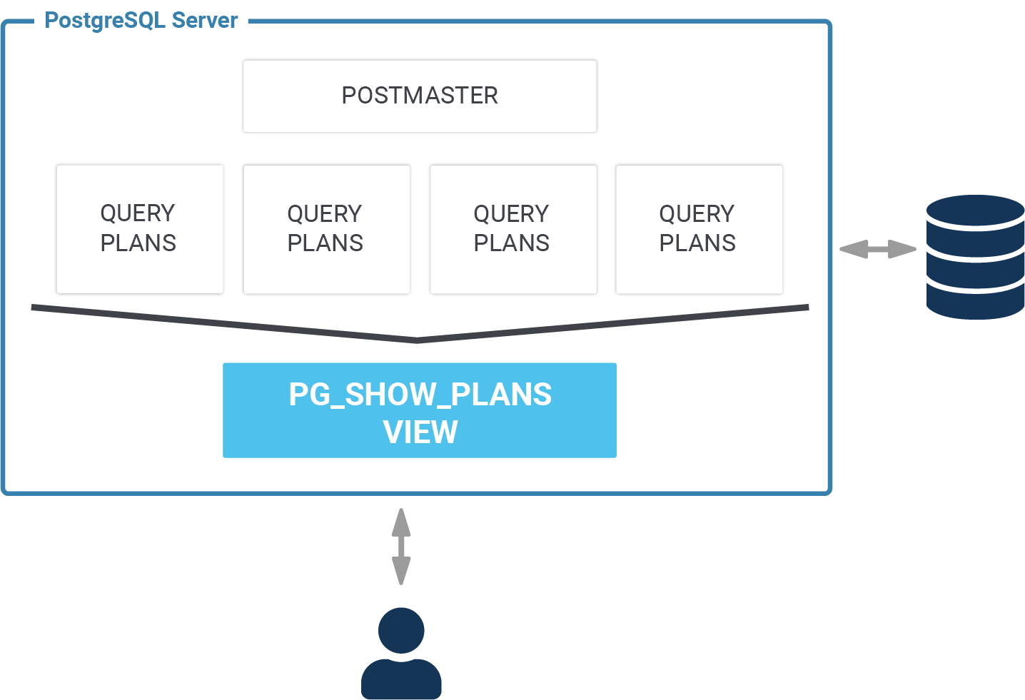
After 20 years in professional PostgreSQL support and consulting we are finally able to answer one of the most frequently asked questions: “How can I see all active query/ execution plans?" Ladies and gentlemen, let me introduce you to pg_show_plans, an extension which does exactly that. pg_show_plans is Open Source and can be used free of charge as a standard PostgreSQL extension. It will help people to diagnose problems more efficiently and help to digging into more profound performance issues.

How does pg_show_plans work?

pg_show_plans uses a set of hooks in the PostgreSQL core to extract all the relevant information. These plans are then stored in shared memory and exposed via a view. This makes it possible to access these plans in an easy way. 

The performance overhead of pg_show_plans will be discussed in a future blog post. Stay tuned for more information and visit our blog on a regular basis.

Installing pg_show_plans

pg_show_plans is available on GitHub for free and can be used free of charge.

Just clone the GitHub repo:

Then “cd” into the directory and set USE_PGXS. USE_PGXS is important if you want to compile the code outside of the PostgreSQL source tree:

Finally, you can run “make” and “make install”

If things work properly, the code is now successfully installed.

To activate the module, you have to set shared_preload_libraries in postgresql.conf:

Once this is done, the extension can be activated in your database:

Checking execution plans in PostgreSQL

To see how this module works we need two connections: In the first connection I will run a long SQL statement which selects data from a fairly complex system view. To make sure that the query takes forever I have added pg_sleep:

You can now use a second connection to inspect the plan:

pg_show_plans is going to return information for every database connection. Therefore it is possible to see everything at a glance and you can react even before a slow query has ended. As far as we know, pg_show_plans is the only module capable of providing you with this level of detail.

Finally...

If you want to know more about execution plans we suggest checking out one of our other posts dealing with index scans, bitmap index scans and alike.

We are looking forward to seeing you on our blog soon for more interesting stuff. 

 

 

Embedded SQL is by no means a new feature — in fact it is so old-fashioned that many people may not know about it at all. Still, it has lots of advantages for client code written in C. So I'd like to give a brief introduction and talk about its benefits and problems.

What is embedded SQL?

Typically you use a database from application code by calling the API functions or methods of a library. With embedded SQL, you put plain SQL code (decorated with “EXEC SQL”) smack in the middle of your program source. To turn that into correct syntax, you have to run a pre-processor on the code that converts the SQL statements into API function calls. Only then you can compile and run the program.

Embedded SQL is mostly used with old-fashioned compiled languages like C, Fortran, Pascal, PL/I or COBOL, but with SQLJ there is also a Java implementation. One reason for its wide adoption (at least in the past) is that it is specified by the SQL standard ISO/IEC 9075-2 (SQL/Foundation). This enables you to write fairly portable applications.

To be able to discuss the features in some more detail, I'll introduce a sample C program using embedded SQL.

Sample embedded SQL program

The sample program operates on a database table defined like this:

The program is in a file sample.pgc and looks like this:

Embedded SQL syntax explained

Each SQL statement or declaration starts with the magic words EXEC SQL and ends with a semicolon.

Most statements are translated by the preprocessor right where they are.

Connection and disconnection

There are several ways to specify a connect string to the database, and of course the value does not have to be hard-coded. You can also use CONNECT TO DEFAULT and use libpq environment variables and a password file to connect.

It is possible to open several database connections at once; then you have to name the connections. Connections are like global variables: they are available everywhere once opened, and you don't have to pass them to functions.

Host variables

Special “host variables” exchange data between the program and the SQL statements.

They have to be declared in the declare section:

This is just like any other C variable declaration, but only these variables can be used in SQL statements. They have to be prepended with a colon (:) in SQL statements:

The last variable, v_val_ind, is an indicator variable: it is set to a negative number to indicate a NULL value.

One advantage of embedded SQL is that the conversion between PostgreSQL data types and C data types is done automatically. With libpq, you can either get strings or the internal PostgreSQL representation. There is the additional (non-standard) libpgtypes library that provides convenient support for data types like timestamp or numeric.

Note that v_val was declared as char[81] so that it can contain any 20 UTF-8 characters. If you cannot predict the size of the result, you can use descriptor areas to exchange data.

Exception handling

If SQL statements cause an error or warning or return no data, you define the program behavior with WHENEVER declarations:

These slightly diverge from the SQL standard, which only has CONTINUE and GO TO label actions. Also, the standard uses SQLEXCEPTION instead of SQLERROR. The DO BREAK action inserts a break; statement to break out of the containing loop.

Different from other embedded SQL statements, these directives apply to all embedded SQL statements below them in the source file. They define how the pre-processor translates SQL statements and are independent of the control flow in the program.

To avoid recursion, it is best to set the action to CONTINUE (ignore) in the exception handler.

Note that this syntax allows to write code without adding error handling to every database call, which is convenient and makes the code concise and readable.

Interplay of embedded SQL with libpq

Some advanced or PostgreSQL-specific features of libpq are not available in embedded SQL, for example the Large Object API or, more importantly, COPY.

To use these, you can call the function ECPGget_PGconn(const char *connection_name), which returns the underlying libpq connection object.

Building the executable

The pre-processor is called ecpg and part of the PostgreSQL core distribution. By default, ecpg assumes that source files have the extension .pgc.

To compile the resulting C program, you can use any C compiler, and you have to link with the libecpg library.

Here is a Makefile that can be used to build the sample program with PostgreSQL v12 on RedHat-like systems:

Conclusion

We have only scratched the surface, but I hope I could demonstrate that embedded SQL is a convenient way of writing database client code in C.

Here is a list of advantages and disadvantages of embedded SQL compared to directly using the C API of libpq:

Disadvantages:

• requires preprocessing
• unknown to most present-day developers
• less powerful than libpq (e.g., no direct COPY support)

Advantages:

• standardized API for good portability between databases
• more concise and readable code
• simple but elegant exception handling
• translation between C and SQL data types

pg_timetable: Advanced PostgreSQL cron-like scheduler released!

Hello there, this is your developer speaking...

I'm struggling with how to start this post, since I've procrastinated a lot. There should be at least 5 published posts on this topic already. But there is only one by Hans-Jürgen Schönig. I'm thanking him for trying to cover my back, but the time has come!

Major release? But why version 2?

Well, that's a tricky question. We've started working on pg_timetable a year ago, aiming our own targets. Then we've found out that this project might be interesting for other people and we opened it.

Soon we received some feedback from users and improved our product. There were no releases and versions at that time. But suddenly, we faced a situation where you cannot grow or fix anything vital, until you introduce changes in your database schema. Since we are not a proprietary project anymore, we must provide back-compatibility for current users.

Precisely at this time, you understand that there is a need for releases (versions) and database migrations to the new versions.

Major versions usually change the internal format of system tables and data representation. That's why we go for the new major version 2, considering the initial schema as version 1.

This means that, if you have a working installation of the pg_timetable, you will need to use --upgrade command-line option, but don't forget to make a backup beforehand.

So what are those dramatic changes?

Brand new cron-style schedules

How scheduling information was stored before:

Turned out, it's incredibly inconvenient to store schedules one job per line because of the UI. Consider this simple cron syntax:
0 */6 * * * which stands for "every 6th hour".

So in the old model, it will produce 4 rows for hours 6, 12, 18, 24.

It's not a problem for the database itself to store and work with a large number of rows. However, now if a user wants to update the schedule, he/she either must update each entrance row by row or delete old rows and insert new ones.

So we've come out with the new syntax:

@reboot, @every, and @after jobs

To be honest, these guys are the main reasons why we've changed the database schema. 🙂

If a job is marked as @reboot, it will be executed once after pg_timetable connects to the database or after connection reestablishment.

This kind of job is useful for initialization or for clean-up actions. Consider to remove leftovers from the unfinished tasks, e.g., delete downloaded or temporary files, clean tables, reinitialize schema, etc. One may rotate the log of the previous session, backup something, send logs by email.

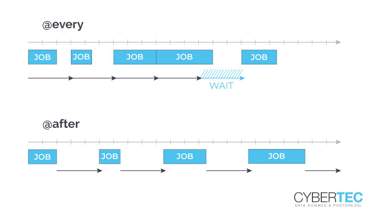
@every and @after are interval tasks, meaning they are not scheduled for a particular time but will be executed repeatedly. The syntax consists of the keyword (@every or @after) followed by proper interval type value.

The only difference is that @every task will be repeated within at equal intervals of time. In contrast, @after task will repeat itself in an interval only after the previous job was finished. See the figure below for details.

 

Here is the list of possible syntaxes:

--no-shell-tasks command line parameter

We've added a startup option that forbids the execution of shell tasks. The reason is simple. If you are in a cloud deployment, you probably won't like shell tasks.

Ants Aasma, Cybertec expert:

 

Linux container infrastructure is basically taking a sieve and trying to make it watertight. It has a history of security holes. So unless you do something like KubeVirt, somebody is going to break out of the container.
Even with KubeVirt, you have to keep an eye out for things like Spectre that can break through the virtualization layer.
It's not the database we are worried about in this case. It's other people's databases running on the same infrastructure.

Release packages

Starting on this release, we will provide you with pre-built binaries and packages. Currently, we build binaries:

• for x86 and x64 platforms;
• for Linux, macOS, and Windows operating systems;
• packed into .rpm and .deb packages;
• available in .zip and .tar.gz archives.

We consider including our packages into official Yum and Apt PostgreSQL repositories.

Continuous testing

And last but not least! Continuous testing was implemented using GitHub Actions, meaning all pull requests and commits are checked automatically to facilitate the development and integration of all kinds of contributors.

Cheers!

When designing a database application, the layout of data in disk is often neglected. However, the way data is clustered by PostgreSQL can have a major performance impact. Therefore it makes sense to take a look at what can be done to improve speed and throughput. In this post you will learn one of the most important tricks.

PostgreSQL: To sort or not to sort

To demonstrate the importance of the on-disk layout I have created a simple test set:

Note that both data sets are absolutely identical. I have loaded 10 million rows into a simple table. However, in the first case data has been sorted, then inserted. generate_series returns data in ascending order and because the table is new data will be written to disk in that order.
In the second case I decided to shuffle the data before insertion. We are still talking about the same data set. However, it is not in the same order:

In both cases the size on disk is the same. There are no changes in terms of space consumption which can be an important factor as well.

Creating an index in PostgreSQL

Let us create an index on both tables:

Even creating the index is already faster on sorted data for various reasons. However, creating initial indexes does not happen too often, so you should not worry too much.

In the next step we can already create optimizer statistics and make sure that all hint bits are set to ensure a fair performance comparison:

Reading blocks of database

Now that all the test data sets are in place we can run a simple test: Let us fetch 49000 rows from the sorted data set first:

Not bad. We need 11.785 milliseconds to read the data. What is most important to consider here is that the number of 8k blocks needed is 138, which is not much. “shared hit” means that all the data has come from memory.

Let me run the same test again:

In this case the query took a bit longer: 13.4 ms. However, let us talk about the most important number here: The number of blocks needed to return this result. 18799 blocks. Wow. That is roughly 150 times more.

One could argue that the query is not really that much slower. This is true. However, in my example all data is coming from memory. Let us assume for a moment that data has to be read from disk because for some reason we get no cache hits. The situation would change dramatically. Let us assume that reading one block from disk takes 0.1 ms:

138 * 0.1 + 11.7 = 25.5 ms
vs.
18799 * 0.1 + 13.4 = 1893.3 ms

That is a major difference. This is why the number of blocks does make a difference – even if it might not appear to be the case at first glance. The lower your cache hit rates are, the bigger the problem will become.

There is one more aspect to consider in this example: Note that if you want to read a handful of rows only the on-disk layout does not make too much of a difference. However, if the subset of data contains thousands of rows, the way is ordered on disk does have an impact on performance.

CLUSTER: PostgreSQL comes to the rescue

The CLUSTER command has been introduced many years ago to address exactly the issues I have just outlined. It allows you to organize data according to an index. Here is the syntax:

URL: https://www.postgresql.org/docs/12/sql-cluster.html

Utilizing the CLUSTER command is easy. The following code snipped will show how you can do that:

To see what happens I have executed the same query as before again. However, there is something important to be seen:

PostgreSQL has changed the execution plan. This happens due to wrong statistics. Therefore it is important to run ANALYZE to make sure that the optimizer has up-to date information:

Once the new optimizer statistics is in place the execution plan will be as expected again:

Maintaining order

If you have decided to cluster a table it does NOT mean that order on disk is maintained forever. If you run UPDATES etc. frequently the table might gradually loose order again. Therefore, CLUSTER is especially useful if your data is rather static. It can also make sense to order data as you import it to ensure physical order.

Finally …

If you want to learn more about database performance and storage consider checking out my post about shrinking the storage footprint of PostgreSQL.

---

In order to receive regular updates on important changes in PostgreSQL, subscribe to our newsletter, or follow us on Facebook or LinkedIn.

 

(Last updated on 2023-01-24) Recently, while troubleshooting PostgreSQL performance problems, I ran into problems with subtransactions twice. So I thought this was a nice topic for another blog post.

What are subtransactions?

Everybody knows database transactions. In PostgreSQL, which is operating in autocommit mode, you have to start a transaction that spans multiple statements explicitly with BEGIN or START TRANSACTION and close it with END or COMMIT. If you abort the transaction with ROLLBACK (or end the database session without committing) all work done inside the transaction becomes undone.

Now subtransactions allow you to roll back part of the work done in a transaction. You start a subtransaction inside a transaction with the standard SQL statement:

“name” is an identifier (no single quotes!) for the subtransaction. You cannot commit a subtransaction in SQL (it is automatically committed with the transaction that contains it), but you can roll it back with:

The use of subtransactions

Subtransactions are useful in longer transactions. In PostgreSQL, any error inside a transaction will abort the transaction:

With a transaction that does a lot of work this is quite annoying, because it means that all work done so far is lost. Subtransactions can help you recover from such a situation:

Note that ROLLBACK TO SAVEPOINT starts another subtransaction called a when it rolls back the old one.

Subtransactions in PL/pgSQL

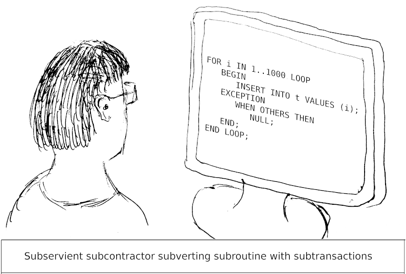
Even if you have never used the SAVEPOINT statement, you may already have encountered subtransactions. Written in PL/pgSQL, the code in the previous section looks like this:

Every time you enter a block with an EXCEPTION clause, a new subtransaction is started. The subtransaction is committed when you leave the block, and rolled back when you enter the exception handler.

Compatibility with other databases

Many other databases handle errors inside a transaction differently. Rather than aborting the complete transaction, they roll back only the statement that caused the error, leaving the transaction itself active.

When migrating or porting from such a database to PostgreSQL, you might be tempted to wrap every single statement in a subtransaction to emulate the above behavior.

The PostgreSQL JDBC driver even has a connection parameter “autosave” that you can set to “always” to automatically set a savepoint before each statement and rollback in case of failure.

As the following will show, this alluring technique will lead to serious performance problems.

A performance test case

To demonstrate the problems caused by overuse of subtransactions, I created a test table:

The table is small, unlogged and has a low fillfactor to reduce the required I/O as much as possible. This way, I can observe the effects of subtransactions better.

I'll use pgbench, the benchmarking tool shipped with PostgreSQL, to run the following custom SQL script:

The script will set 60 savepoints for test number 1, and 90 for test number 2. It uses prepared statements to minimize the overhead of query parsing.

pgbench will replace :client_id with a number unique to the database session. So as long as there are no more than 10 clients, each client's UPDATEs won't collide with those of other clients, but they will SELECT each other's rows.

Running the performance test

Since my machine has 8 cores, I'll run the tests with 6 concurrent clients for ten minutes.

To see meaningful information with “perf top”, you need the PostgreSQL debugging symbols installed. This is particularly recommended on production systems.

Test 1 (60 subtransactions)

This is what “perf top --no-children --call-graph=fp --dsos=/usr/pgsql-12/bin/postgres” shows while the test is running:

Test 2 (90 subtransactions)

This is what “perf top --no-children --call-graph=fp --dsos=/usr/pgsql-12/bin/postgres” has to say:

Even if we take into account that the transactions in test 2 are one longer, this is still a performance regression of 60% compared with test 1.

Implementation of subtransactions

To understand what is going on, we have to understand how transactions and subtransactions are implemented.

Whenever a transaction or subtransaction modifies data, it is assigned a transaction ID. PostgreSQL keeps track of these transaction IDs in the commit log, which is persisted in the pg_xact subdirectory of the data directory.

However, there are some differences between transactions and subtransactions:

• Each subtransaction has a containing transaction or subtransaction (the “parent”)
• Committing a subtransaction does not require a WAL flush
• There can be only one transaction per database session, but many subtransactions

The information which (sub)transaction is the parent of a given subtransaction is persisted in the pg_subtrans subdirectory of the data directory. Since this information becomes obsolete as soon as the containing transaction has ended, this data do not have to be preserved across a shutdown or crash.

Subtransactions and visibility

The visibility of a row version (“tuple”) in PostgreSQL is determined by the xmin and xmax system columns, which contain the transaction ID of the creating and destroying transactions. If the transaction ID stored is that of a subtransaction, PostgreSQL also has to consult the state of the containing (sub)transaction to determine if the transaction ID is valid or not.

To determine which tuples a statement can see, PostgreSQL takes a snapshot of the database at the beginning of the statement (or the transaction). Such a snapshot consists of:

• a maximum transaction ID: everything from that transaction on is invisible
• the list of transactions and subtransactions that were active when the snapshot was taken
• the command number of the earliest visible command in the current (sub)transaction

A snapshot is initialized by looking at the process array, which is stored in shared memory and contains information about all currently running backends. This, of course, contains the current transaction ID of the backend and has room for at most 64 non-aborted subtransactions per session. If there are more than 64 such subtransactions, the snapshot is marked as suboverflowed.

Explaining the test results

A suboverflowed snapshot does not contain all data required to determine visibility, so PostgreSQL will occasionally have to resort to pg_subtrans. These pages are cached in shared buffers, but you can see the overhead of looking them up in the high rank of SimpleLruReadPage_ReadOnly in the perf output. Other transactions have to update pg_subtrans to register subtransactions, and you can see in the perf output how they vie for lightweight locks with the readers.

Diagnosing the problem of too many subtransactions

Apart from looking at “perf top”, there are other symptoms that point at the direction of this problem:

• Your workload performs well when run single-threaded, but badly when run in several concurrent database sessions
• You often see the wait event “SubtransSLRU” (“SubtransControlLock” in older releases) in pg_stat_activity
• From PostgreSQL v13 on, you can look at the monitoring view pg_stat_slru and check if blks_read in the row with name = 'Subtrans' keeps growing. That indicates that PostgreSQL has to read disk pages because it needs to access subtransactions that are no longer cached.
• If you export a snapshot using the “pg_export_snapshot()” function, the resulting file in the pg_snapshots subdirectory of the data directory will contain the line “sof:1” to indicate that the subtransaction array overflowed
• From PostgreSQL v16 on, you can call the function pg_stat_get_backend_subxact(integer) to return the number of subtransactions for a backend process and whether the subtransaction cache overflowed or not

Conclusion

Subtransactions are a great tool, but you should use them wisely. If you need concurrency, don't start more than 64 subtransactions per transaction.

The diagnostics shown in this article should help you determine whether you are suffering from the problem, or not.

Finding the cause of that problem can be tricky. For example, it may not be obvious that a function with an exception handler that you call for each result row of an SQL statement (perhaps in a trigger) starts a new subtransaction.

 

---

In order to receive regular updates on important changes in PostgreSQL, subscribe to our newsletter, or follow us on Twitter, Facebook, or LinkedIn.

If you are running PostgreSQL in production you might have already noticed that adjusting checkpoints can be a very beneficial thing to tune the server and to improve database performance overall. However, there is more to this: Increasing checkpoint distances can also help to actually reduce the amount of WAL that is created in the first place. That is right. It is not just a performance issue, but it also has an impact on the volume of log created.

You want to know why? Let us take a closer look!

Creating a test installation

For my test I am using a normal PostgreSQL 12 installation. To do that I am running initdb by hand:

Then I have adjusted two parameters in postgresql.conf:

and restarted the server:

First of all I have reduced max_wal_size to make sure that PostgreSQL checkpoint a lot more often than this would be the case in the default installation. Performance will drop like a stone. The second parameter is to tell PostgreSQL to use asynchronous commits. This does not impact WAL generation but will simply speed up the benchmark to get results faster.

Finally I am using pgbench to create a test database containing 10 million rows (= 100 x 100.000)

Running a PostgreSQL benchmark

Let us run a test now: We want to run 10 x 1 million transactions. If you want to repeat the tests on your database make sure the test runs long enough. Let us take a look at the test!

As you can see we managed to run roughly 13.700 transactions per second (on my personal laptop). Let us take a look at the amount of WAL created:

The way to figure out the current WAL position is to call the pg_current_insert_lsn() function. To most people this format might be incomprehensible and therefore it is easier to transform the value into a readable number:

 The pg_size_pretty() function will return the number in a readily understandable format:

Increasing checkpoint distances

Let us stop the database, delete the data directory and initialize it again. This time my postgresql.conf parameters will be set to way higher values:

 Then we start the database again, populate it with data and run pgbench with the exact same parameters. Keep in mind that to repeat the process it is necessary to run a fixed number of transactions instead of running the test for a certain time. This way we can fairly compare the amount of WAL created.

Let us take a look and see how much WAL has been created this time:

Wow, only 5.3 GB of WAL. This is a major improvement but why did it happen?

Understanding WAL creation

The idea of the transaction log is to make sure that in case of a crash the system will be able to recover nicely. However, PostgreSQL cannot keep the transaction log around forever. The purpose of a checkpoint is ensuring that all data is safe in the data file before the WAL can be removed from disk.

Here comes the trick: If a block is modified after a checkpoint for the first time it has to be logged completely. The entire block will be written to the WAL. Every additional change does not require the entire block to be written – only the changes have to be logged which is, of course, a lot less.

This is the reason for the major difference we see here. By increasing the checkpoint distances to a really high value, we basically reduced checkpoints to an absolute minimum which in turn reduces the number of “first blocks” written.

Changing WAL settings is not just good for performance in the long run – it will also reduce the volume of WAL.

Further reading

If you want to know more about PostgreSQL and want to learn something about VACUUM check out my blog about this important topic.

Also, if you like our posts you might want to share them on LinkedIn or on Facebook. We are looking forward to your comments.