PostgreSQL replication (synchronous and asynchronous replication) is one of the most widespread features in the database community. Nowadays, people are building high-availability clusters or use replication to create read-only replicas to spread out the workload. What is important to note here is that if you are using replication, you must make sure that your clusters are properly monitored.
The purpose of this post is to explain some of the fundamentals, to make sure that your PostgreSQL clusters stay healthy.

pg_stat_replication: Inspecting the current state

The best way to monitor replication is to use pg_stat_replication, which contains a lot of vital information. Here is what the view looks like:

The number of columns in this view has grown substantially over the years. However, let’s discuss some fundamentals first.

pg_stat_replication: WAL sender information

People often say that pg_stat_replication is on the “primary”. That’s not quite true. What the view does is to expose information about the wal_sender process. In other words: if you are running cascaded replication, it means that a secondary might also show entries in case it replicates to further slaves. Here is an image illustrating the situation:

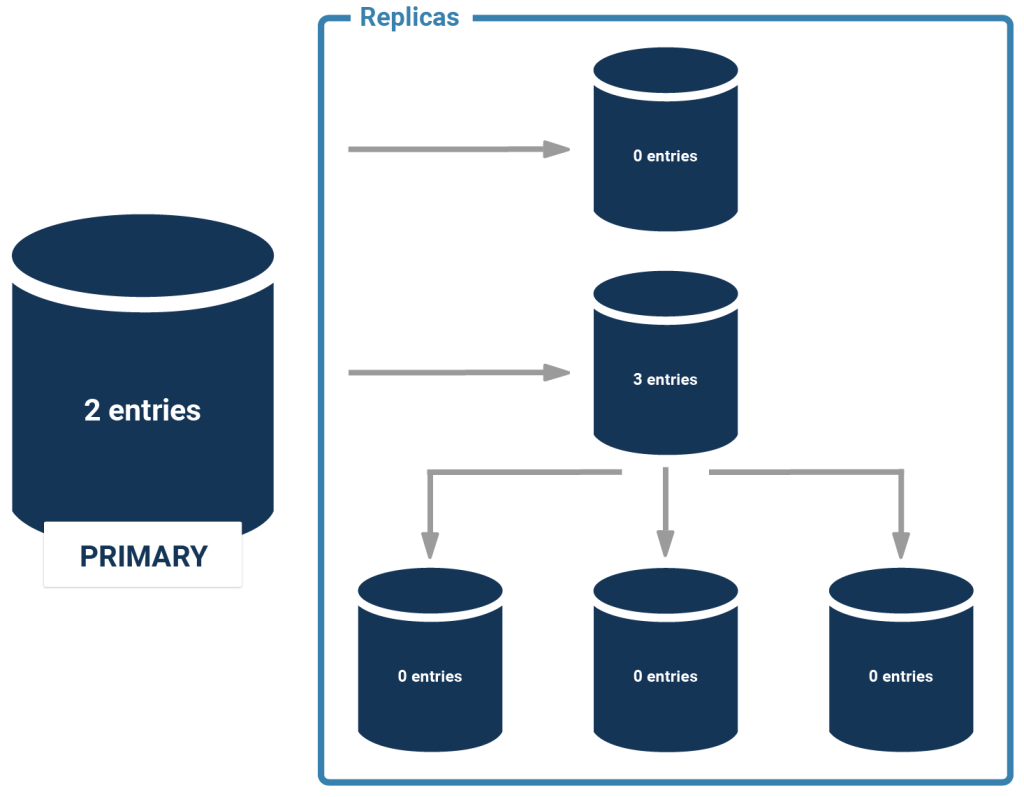
For every WAL sender process you will get exactly one entry. What is important is that each server is only going to see the next ones in the chain - a sending server is never going to see “through” a slave. In other words: In the case of cascading replication, you have to ask every sending server to get an overview.

But there’s more: often people have to determine if a slave is up to date or not. There are various things which are relevant here:

• sent_lsn: How much WAL has been sent over the network already?
• write_lsn: How much WAL has been sent to the operating system? (without flushing)
• flush_lsn: How much WAL has been flushed to disk already?
• replay_lsn: How much WAL has been replayed and is therefore visible to queries?

The following picture illustrates those fields:

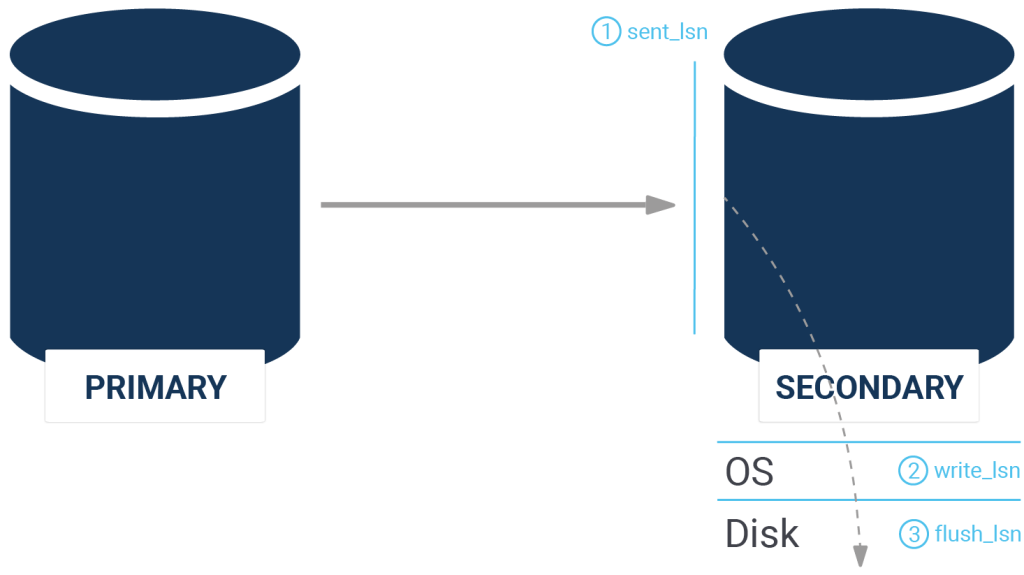
What’s important to note here is that PostgreSQL offers a special data type to represent this data: pg_lsn
One can figure out the current WAL position easily. Here is how it works:

What’s noteworthy here is that it’s possible to make calculations:

PostgreSQL provides various operators to do such calculations. In other words: it’s easy to figure out how far a replica has fallen behind.

flush_lsn vs. replay_lsn

People keep asking us what the difference between the flush_lsn and the replay_lsn might be. Well, let’s dig in and find out: when WAL is flowing from the master to the slave, it is first sent over the network, then sent to the operating system and finally transactions are flushed to disk to assure durability (= crash safety). The flush_lsn obviously represents the last WAL position flushed to disk. The question now is: is data visible as soon as it is flushed? The answer is: no, there might be replication conflicts as described in one of our older blog posts. In case of a replication conflict, the WAL is persisted on the replica - but it is only replayed when the conflict is resolved. In other words, it might happen that data is stored on the slave which is not yet replayed and thus accessible by end users.

This is important to note, because replication conflicts occur more often than you might think. If you see a message as follows, you have hit a replication conflict:

Replication lags

Sometimes it’s necessary to determine the amount of replication lag in seconds. So far, we have seen the distance between two servers in bytes. If you want to measure the lag, you can take a look at the _lag columns. The data type of those columns is “interval” so you can see what the delay is in seconds or even minutes. If replication is working properly, the lag is usually very very small (milliseconds). However, you might want to monitor that.

A word of caution: if you are running large scale imports such as VACUUM or some other expensive operations, it might easily happen that the disk throughput is higher than the network bandwidth. In this case, it is possible and quite likely that the slave falls behind. You have to tolerate that and make sure that alerting does not kick in too early.

pgwatch2: Ready made tooling

To monitor replication, you can rely on the manual magic I have just shown. However, there is also a lot of ready-made tooling out there to facilitate this task. One of the things we can recommend is pgwatch2, which can be downloaded for free as a container.

If you want to check out a demo showing how pgwatch works, consider checking out our pgwatch2 website >>.

Finally …

If you want to learn more about PostgreSQL in general we recommend to check out some of our other posts. In case you are interested in storage you may want to take a look at one of our posts about pgsqueeze.
 

---

In order to receive regular updates on important changes in PostgreSQL, subscribe to our newsletter, or follow us on Twitter, Facebook, or LinkedIn.

By Kaarel Moppel: So, you’re building the next unicorn startup and are thinking feverishly about a future-proof PostgreSQL architecture to house your bytes? My advice here, having seen dozens of hopelessly over-engineered / oversized solutions as a database consultant over the last 5 years, is short and blunt: Don’t overthink, and keep it simple on the database side! Instead of getting fancy with the database, focus on your application. Turn your microscope to the database only when the need actually arises, m'kay! When that day comes, first of all, try all the common vertical scale-up approaches and tricks. Try to avoid using derivative Postgres products, or employing distributed approaches, or home-brewed sharding at all costs - until you have, say, less than 1 year of breathing room available.

Wow, what kind of advice is that for 2021? I’m talking about a simple, single-node approach in the age of Big Data and hyper-scalability...I surely must be a Luddite or just still dizzy from too much New Year’s Eve champagne. Well, perhaps so, but let’s start from a bit further back...

PostgreSQL and MySQL - brothers from another mother grow up - scaling

Over the holidays, I finally had a bit of time to catch up on my tech reading / watching TODO-list (still dozens of items left though, arghh)...and one pretty good talk was on the past and current state of distributed MySQL architectures by Peter Zaitsev of Percona. Oh, MySQL??? No no, we haven’t changed “horses” suddenly, PostgreSQL is still our main focus 🙂 It’s just that in many key points pertaining to scaling, the same constraints actually also apply to PostgreSQL. After all, they’re both designed as single-node relational database management engines.

In short, I’m summarizing some ideas out of the talk, plus adding some of my own. I would like to provide some food for thought to those who are overly worried about database performance - thus prematurely latching onto some overly complex architectures. In doing so, the “worriers” sacrifice some other good properties of single-node databases - like usability, and being bullet-proof.

All distributed systems are inherently complex, and difficult to get right

If you’re new to this realm, just trust me on the above, OK? There’s a bunch of abandoned or stale projects which have tried to offer some fully or semi-automatically scalable, highly available, easy-to-use and easy-to-manage DBMS...and failed! It’s not an utterly bad thing to try though, since we can learn from it. Actually, some products are getting pretty close to the Holy Grail of distributed SQL databases (CockroachDB comes to mind first). However, I’m afraid we still have to live with the CAP theorem. Also, remember that to go from covering 99.9% of corner cases of complex architectures to covering 99.99% is not a matter of linear complexity/cost, but rather exponential complexity/cost!

Although after a certain amount of time a company like Facebook surely needs some kind of horizontal scaling, maybe you’re not there yet, and maybe stock Postgres can still provide you some years of stress-free cohabitation. Consider: Do you even have a runway for that long?

What does plain PostgreSQL offer?

* A single PostgreSQL instance can easily do hundreds of thousands of transactions per second

For example, on my (pretty average) workstation, I can do ca. 25k simple read transactions per 1 CPU core on an “in memory” pgbench dataset...with the default config for Postgres v13! With some tuning (by the way, tuning reads is much harder in Postgres than tuning writes!) I was able to increase it to ~32k TPS per core, meaning: a top-notch, dedicated hardware server can do about 1 million short reads! With reads, you can also usually employ replicas - so multiply that by 10 if needed! You then need to somehow solve the query routing problem, but there are tools for that. In some cases, the new standard LibPQ connection string syntax (target_session_attrs) can be used - with some shuffling. By the way, Postgres doesn’t limit the number of replicas, though I personally have never witnessed more than 10 replicas. With some cascading, I’m sure you could run dozens without bigger issues.

* A single node can typically do tens of thousands of write transactions per second

On my humble workstation with 6 cores (12 logical CPUs) and NVMe SSD storage, the default very write-heavy (3 UPD, 1 INS, 1 SEL) “pgbench” test greets me with a number of around 45k TPS - for example, after some checkpoint tuning - and there are even more tuning tricks available.

* A single Postgres instance can easily handle dozens of Terabytes of data

Given that you have separated “hot” and “cold” data sets, and there’s some thought put into indexing, etc., a single Postgres instance can cope with quite a lot of data. Backups and standby server provisioning, etc. will be a pain, since you’ll surely meet some physical limits even on the finest hardware. However, these issues are common to all database systems. From the query performance side, there is no reason why it should suddenly be forced to slow down!

* A single node instance is literally bullet-proof as far as data consistency is concerned

Given that 1) you declare your constraints correctly, 2) don’t fool around with some “fsync” or asynchronous commit settings, and 3) your disks don’t explode, a single node instance provides rock-solid data consistency. Again, the last item applies to any data storage, so hopefully, you have “some” backups somewhere...

* Failures are easily comprehensible - thus also recoverable

Meaning: that even if something very bad happens and the primary node is down, the worst outcome is that your application is just currently unavailable. Once you do your recovery magic (or better, let some bot like Patroni take care of that) you’re exactly where you were previously. Now compare that with some partial failure scenarios or data hashing errors in a distributed world! Believe me, when working with critical data, in a lot of cases it’s better to have a short downtime than to have to sort out some runaway datasets for days or weeks to come, which is confusing for yourself and your customers.

Tips to be prepared for scaling

In the beginning of the post, I said that when starting out, you shouldn’t worry too much about scaling from the architectural side. That doesn’t mean that you should ignore some common best practices, in case scaling could theoretically be required later. Some of them might be:

* Don’t be afraid to run your own database

This might be the most important thing on the list - with modern real hardware (or some metal cloud instances) and the full power of config and filesystem tuning and extensions, you’ll typically do just fine on a single node for years. Remember that if you get tired of running your own setup, nowadays you can always migrate to some cloud providers - with minimal downtime - via Logical Replication! If you want to know how, see here. Note that I specifically mentioned “real” hardware above, due to the common misconception that a single cloud vCPU is pretty much equal to a real one...the reality is far from that of course - my own impression over the years has been that there is around a 2-3x performance difference, depending on the provider/region/luck factor in question.

* Try to avoid the serious mistake of having your data "architecture" centered around a single huge table

You’d be surprised how often we see that...so slice and dice early, or set up some partitioning. Partitioning will also do a lot of good to the long-term health of the database, since it allows multiple autovacuum workers on the same logical table, and it can speed up IO considerably on enterprise storage. If IO indeed becomes a bottleneck at some point, you can employ Postgres native remote partitions, so that some older data lives on another node.

* Make sure to “bake in” a proper sharding key for your tables/databases

Initially, the data can just reside on a single physical node. If your data model revolves around the “millions of independent clients” concept for example, then it might even be best to start with many “sharded” databases with identical schemas, so that transferring out the shards to separate hardware nodes will be a piece of cake in the future.

To conclude

There are benefits to systems that can scale 1000x from day one...but in many cases, there’s also an unreasonable (and costly) desire to be ready for scaling. I get it, it’s very human - I’m also tempted to buy a nice BMW convertible with a maximum speed of 250 kilometers per hour...only to discover that the maximum allowed speed in my country is 110, and even that during the summer months.

The thing that resonated with me from the Youtube talk the most was that there’s a definite downside to such theoretical scaling capability - it throttles development velocity and operational management efficiency at early stages! Having a plain rock-solid database that you know well, and which also actually performs well - if you know how to use it - is most often a great place to start with.

By the way, here’s another good link on a similar note from a nice Github collection and also one pretty detailed overview here about how an Alexa top 250 company managed to get by with a single database for 12 years before needing drastic scaling action!

To sum it all up: this is probably a good place to quote the classics: premature optimization is the root of all evil…

As CYBERTEC keeps expanding, we need a lot more office space than we previously did. Right now, we have a solution in the works: a new office building. We wanted something beautiful, so we started to dig into mathematical proportions to achieve a reasonable level of beauty. We hoped to make the building not just usable, but also to have it liked by our staff.

I stumbled upon some old books about proportions in architecture and went to work. Fortunately, one can use PostgreSQL to do some of the more basic calculations needed.

Basic rules for beauty

This is of course a post about PostgreSQL, and not about architecture-- but let me explain a very basic concept: golden proportions. Beauty is not random; it tends to follow some mathematical rules. The same is true in music. “Golden proportions” are a common concept: Let’s take a look:

We are looking at a magic number here: 1.618. It has some nice attributes. If we invert it is basically “magic number - 1”. If we square it, what we get is “magic number + 1”. If we take a line and break it up into two segments we can use 1 : 1.618. Humans will tend to find this more beautiful than splitting the line using 1 : 1.8976 or so.
Naturally we can make use of this wisdom to create a basic rectangle:

In the case of our new building, we decided to use the following size:

The basic layout is 16 x 26 meters. It matches all mathematical proportions required in the basic layout.

Inlining a semi-circle

To make the building look more appealing, we decided to add a small semi-circle to the rectangle. The question is: What is the ideal diameter of the semi-circle? We can use the same formula as before:

I have used a CTE (common table expression) here. PostgreSQL 13 has a nice feature to handle those expressions. Let’s take a look at the execution plan:

The optimizer has inlined the expression. What we get is:

Then, the optimizer does “constant” folding. All that is left in the execution plan is a “result” node which just displays the answer. The CTE has been removed from the plan entirely.

Making the front of the building more interesting

To make sure the front of the building is not too boring, we need to figure out which numbers are “allowed” and which ones are not. The way to do that is to use recursion:

The idea is to make sure that all components are related to all other components. What we do here is start with 26 meters and calculate the “long” and the “short sides”. Then we use this input for the next iteration, so that we can get a series of valid numbers which guarantee that things fit perfectly. Fortunately, PostgreSQL can do recursion in a nice, ANSI-compatible way. Inside the WITH the first SELECT will assign the start values of the recursion. Then the second part after the UNION ALL will call the recursion which is terminated by the WHERE-clause. At the end of the day, we get a sequence of mathematically correct numbers.

However, once in a while you want to see which iteration a line belongs to. Here is how this can be achieved:

row_number() is a function returning a simple number indicating the line we are looking at.

More good numbers

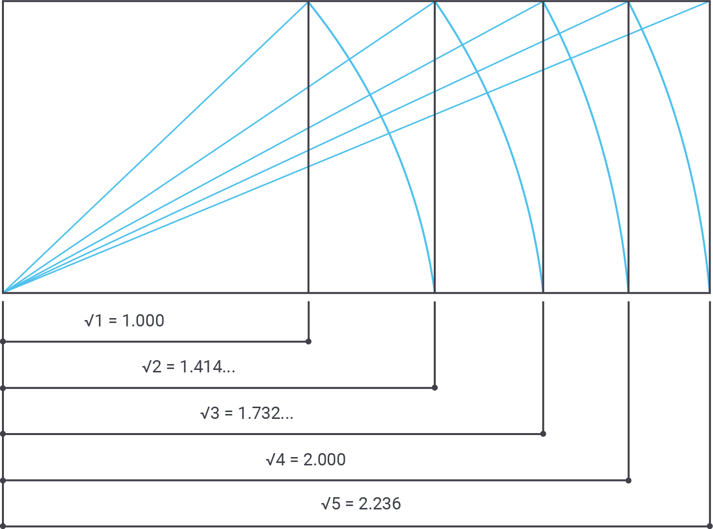
However, there are more “good” numbers in architecture than golden proportions. Square roots and so on are also important. To help calculate those numbers one can use a function:

Golden proportions are a good thing. However, sometimes it is not possible to use those numbers alone. If we look at some of the greatest buildings (Pantheon, etc.) in the world, we will see that the architects also worked with square roots, cubic roots and so on.

The way to do that in PostgreSQL is to use a function. However, in this case we want a function to return more than just one field. The solution to the problem is a composite data type. It can return more than just one value.

22, 27m, and 35m meters are obviously correct values which we can use to ensure beauty.

What you see is that we have used the function call for one number. However, sometimes you might want to calculate things for many values. To do that, it is important to understand how you can handle the return value of composite types:

As you can see, “a” can be used in the SELECT-clause (“target list”) directly. The result is not that readily readable-- however, it is possible to expand this field and extract individual columns as shown in the next listing:

This opens the door to calculate our numbers for an entire series of numbers:

All we did was to pass the “id” to the function and expand those columns.

Finally …

If you want to learn more about upgrading PostgreSQL, you should check out our blog post about logical replication >>

I decided to start out this year by looking into my notes from last year and extracting from them a small set of Postgres tips for you. This might not be, strictly speaking, fresh news... but I guess the average RAM of tech workers is about 64KB or so nowadays, so some repetition might not be such a bad thing.

Partial indexes

This is a huge one – and you're really missing out if you've not heard of this feature or are not using it enough... as too often seems to be the case in my daily consulting work! Thus this was the first item on my list from last year. For larger amounts of data, partial indexes can literally be a life-saving trick when your back is already against the wall due to some unexpected increase in workload or disk usage. One of the reasons this feature is relatively unknown is that most other popular DBMS engines don't have it at all, or they call it by another name.

The crux of the thing is super easy to remember – stop indexing the most common values! Since Postgres knows what your data looks like, it does not use the index whenever you search for a value that’s too common! As always, when you reduce indexes, you're not just winning on the storage - you can also avoid the penalties incurred when you're inserting or modifying the data. So: with partial indexes, when a new column contains the most common value, we don't have to go and touch the index at all!

When does a value become “too common”? Sadly, there is no simple rule for this, as it depends on a couple of other config/data layout variables as well as the actual queries themselves - but roughly, starting at about 25-50% of the total rows, Postgres will tend to ignore the indexes.

Here is a small test table with 100 million rows to help you visualize the possible size benefits.

Another tip on partial indexes (to finish off the topic) – usually, another perfect set of candidates are any columns that are left mostly empty, i.e., "NULL". The thing is that unlike Oracle, PostgreSQL has default all-encompassing indexes, so that all the NULL-s are physically stored in the index!

Estimating average row/record size in bytes

Quite often, you will need to evaluate the approximate size of a number of rows of data for capacity planning reasons. In these cases, there are a couple of approaches. The simplest ones consist of looking at the table size and row count and then doing some elementary math. However, the simplest approaches can be too rough and inaccurate – most often due to bloat; another reason could be that some historical data might not have some recently added columns (for example, due to some peculiarities of when Postgres built-in compression kicks in, etc.) The fastest way to get an estimate is to use the EXPLAIN command. EXPLAIN has the information embedded on the "cost" side - but do note that the estimate may use stale statistics, and it's generally pretty inaccurate on "toasted" columns.

So what do you do if you want to estimate the storage size of some recent data accurately?

The function listed below, which answers the question raised above, is a welcome discovery for most people when they see it in action. Probably, not many people know about this due to the somewhat "hidden" function name (naming things is one of the two most difficult problems in computer science 🙂 ), and due to the fact that we're abusing the function - which is expecting a column - by feeding in a whole row! Remember: in Postgres all tables automatically get a virtual table type with all columns that is kind of a "scalar" - if they are not, for example, unpacked with "t.*".

The advantage of this function is that we can exactly specify and inspect the data that we're interested in. It also handles the disk storage side of things like compression and row headers!

Keep in mind that the size determined still does not usually map 1-to-1 to real-life disk usage for larger amounts of data due to good old companions like "bloat" and normal "defragmentation" or "air bubbles". So if you want super-sharp estimates, there's no way around generating some real-life test data. But do use a TEMP or UNLOGGED table if you do so; no need to create a huge WAL spike...especially if you happen to run a bunch of replicas.

Avoiding risk on upgrading older Postgres instances to new major versions

A fun (or maybe sad) fact from the Postgres consulting trenches - most Postgres users are running some pretty darn old versions! One of many reasons behind that is commonly voiced as, “We cannot stop our business for so and so many minutes.” I say - fair enough, minutes are bad...but with Logical Replication (LR) we're talking about seconds!!! It’s no magic, far from it - the built-in LR introduced in v10 couldn't be any simpler! We’ve performed many such migrations. In the vast majority of cases, it worked smoothly - as intended! In some cases, there might be problems if the verification/switchover period is overly prolonged...

In short - with LR, there is really no reason to run some ancient (well, in "internet years" at least 🙂 ) versions. If my article got you curious and you want to learn more about this topic, I'd suggest starting here.

By the way, if you're on some pre v10 instance, but higher or equal to v9.4, then logical upgrades are also possible via a 3rd party plugin called "pglogical", which often worked quite well when I used it some years ago.

Detecting which index types are available for my column type

What if you’re unhappy with your indexing performance? Maybe there are some other more cool index types available for your column? Postgres has a bunch of those, actually...

And that's not all - after declaring some "magic" extensions:

the picture changes to something like that below. Quite a lot of stuff to choose from for our good old integer!

By the way, if you're thinking, “What the hell are all those weird index types? Why should I give them a chance?”, then I would recommend starting here and here.

Inspecting metadata at the speed of light with psql's "gdesc"

Since we are talking about data types...how do we determine what is actually delivered to us by the Postgres engine in tabular format? What type of data is in column XYZ for example?

The thing is that sometimes you get some above-average funky query sent to you where developers are having difficulties with "you might need to add explicit type casts" complaints from the server, converting some end results of a dozen sub-selects and transformations, so that the original column and its data type have already fallen into an abyss. Or, maybe the ORM needs an exact data type specified for your query, but runtime metadata introspection might be a painful task in the programming language at hand.

So here’s a quick tip on how to employ a PostgreSQL DBA's best friend "psql" (sorry, doggos) for that purpose:

This only works starting from v11 of Postgres.

 

Thanks for reading, and hopefully it got you back on track to start learning some new Postgres stuff again in 2021! Check out last years blogpost for more tips.

Data types are an important topic in any relational database. PostgreSQL offers many different types, but not all of them are created equal. Depending on what you are trying to achieve, different column types might be necessary. This post will focus on three important ones: the integer, float and numeric types. Recently, we have seen a couple of support cases related to these topics and I thought it would be worth sharing this information with the public, to ensure that my readers avoid some common pitfalls recently seen in client applications.

Creating sample data

To get started, I’ve created a simple table containing 10 million rows. The data types are used as follows:

After the import, optimizer statistics and hint bits have been set to ensure a fair comparison.

Float vs. numeric

While the purpose of the integer data type is clear, there is an important difference between the numeric type and the float4 / float8 types. Internally, float uses the FPU (floating point unit) of the CPU. This has a couple of implications: Float follows the IEEE 754 standard, which also implies that the rounding rules defined by the standard are followed. While this is totally fine for many data sets, (measurement data, etc.) it is not suitable for handling money.
In the case of money, different rounding rules are needed, which is why numeric is the data type you have to use to handle financial data.

Here’s an example:

As you can see, a floating point number always uses approximations. This is perfectly fine in many cases, but not for money. Your favorite tax collector is not going to like approximations at all; that’s why floating point numbers are totally inadequate.

Performance considerations

However, are there any advantages of numeric over a floating point number? The answer is: Yes, performance …
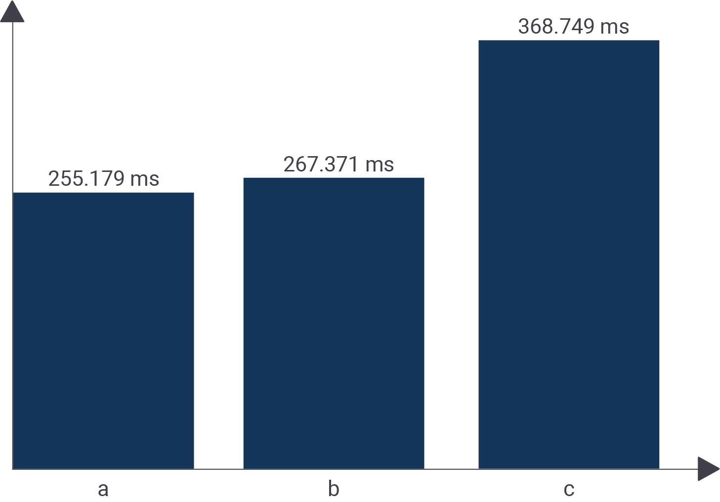
Let us take a look at a simple comparison:

Integer is pretty quick. It executes in roughly 250 ms. The same is true for float4 as you can see in the next listing:

However, the numeric data type is different. There is a lot more overhead, which is clearly visible in our little benchmark:

This query is a lot slower. The reason is the internal representation: “numeric” is done without the FPU and all operations are simulated using integer operations on the CPU. Naturally, that takes longer.

The following image shows the difference:

Finally …

If you want to know more about performance, I can recommend one of our other blog posts about HOT updates.