We are thrilled to announce that the FINAL version of pgwatch2 v1.9 is now ready for your production environment! pgwatch provides a secure, open-source, flexible, self-contained PostgreSQL metrics monitoring/dashboarding solution. pgwatch2 v1.9 supports monitoring PG versions 9.0 to 14 out of the box. Upgrade, or install pgwatch today to see how fantastic it really is. Download it from Github.
pgwatch supports monitoring PostgreSQL versions 9.0 to 14 out of the box
It has been a long time since our previous release. And even though pgwatch2 v1.9 is not considered a major upgrade, there are a lot of impressive changes.
First of all, we have a new maintainer for pgwatch2. That's me, Pavlo Golub. I hope Kaarel Moppel, the author of pgwatch2, will still work on the project - but now without the extra burden of support and maintenance.
We've used the fresh Go v1.17 for all binaries and Docker images.
We now have full PostgreSQL v14 support and support for the latest Grafana v8 visualization solution. For those who still use the previous versions of Grafana, we also added support for v7 and v6 dashboards.
To improve our CI/CD experience and automate some tasks, we've introduced three GitHub Actions in a series of planned workflows:
ReleaseCodeQL analysisClose Stale Issues and PRsRelease workflow will automatically build all artifacts, including Docker images, and publish the release.CodeQL analysis stands guard over code security. It will thoroughly investigate each pull request and each push.
It's not a surprise that many issues are created for open-source projects which never get a follow-up contribution from the topic starter. We have enabled a Close Stale Issues and PRs workflow to keep up with the continuous storm of new issues and PRs. It will mark issues and PRs with no activity as stale, and eventually close them.
We added many more cool features, like new gatherer options, e.g. --try-create-listed-exts-if-missing. Or like new metrics for monitoring "wait_events".
AccessExclusiveLock.--min-db-size-mb flag to ignore "empty" databases. It allows the gatherer to skip measures fetching for empty or for small-sized databases.sqlx.DB from now on.lock_timeout.--no-helper-functions parameter allows you to skip metric definitions which rely on helper functions. This mode makes working with managed instances more fluid, with fewer errors in logs. It uses the SU or superuser version of a metric immediately when available, and not after the first failed call.--emergency-pause-triggerfile flag aims to quickly shut down collectors. The main idea of the feature is to quickly free monitored databases and networks of any extra "monitoring effect" load.You'll find many other new features and improvements in pgwatch2 v1.9. Some may be more important to your use case than those highlighted above. For the latest documentation see here.
sqlx.DB by @kmoppel-cognite in #418release GitHub Action by @pashagolub in #437port parameter from StartPrometheusExporter(), fixes #407 by @pashagolub in #455stale label lower cased by @pashagolub in #457get_table_bloat_approx_sql() when tblpages = 0, closes #464 by @pashagolub in #468Full Changelog: v1.8.5...v1.9.0
See also our new blog about using pgwatch v1.9 with Google Cloud PostgreSQL!
Since my last article about MobilityDB, the overall project has further developed and improved.
This is a very good reason to invest some time and showcase MobilityDB’s rich feature stack by analyzing historical flight data from OpenSky-Network, a non-profit organisation which has been collecting air traffic surveillance data since 2013.
From data preparation and data visualization to analysis – this article covers all the steps needed to quick-start analyzing spatio-temporal data with PostGIS and MobilityDB together.
For a basic introduction to MobilityDB, please check out previous MobilityDB post first.
The article is divided into four sections:
First, you need a current PostgreSQL database, equipped with PostGIS and MobilityDB. I recommend using the latest releases available for your OS of choice, even though MobilityDB works with older releases of PostgreSQL and PostGIS, too. Alternatively, use a docker container from https://registry.hub.docker.com/r/codewit/mobilitydb for those who don’t want to build MobilityDB from scratch.
Second, you'll need a tool to copy our raw flight data served as huge csv files to our database. For this kind of task, I typically use ogr2ogr, a command-line tool shipped with gdal.
Lastly, to visualize our results graphically, we’ll utilize our good old friend “Quantum GIS”, a feature-rich GIS-client, which is available for various operating systems.
The foundation of our analysis is historical flight data, offered by OpenSky-Network free of charge for non-commercial usage. OpenSky offers snapshots of the previous Monday's complete state vector data for the last 6 months. These data sets cover information about time (update interval is one second), icao24, lat/lon, velocity, heading, vertrate, callsign, onground, alert/spi, squawk, baro/geoaltitude, lastposupdate and lastcontact. A detailed description can be found at here.
Enough theory; let’s start by downloading historical datasets for our analysis. The foundation for this post are 24 csv files covering flight data for the day 2022-02-28, which can be downloaded from here.
We’ll continue by creating a new PostgreSQL database, with extensions for PostGIS and MobilityDB enabled. The database will store our state vectors.
|
1 2 3 4 5 6 7 8 9 10 11 12 13 14 15 16 17 |
postgres=# create database flightanalysis; CREATE DATABASE postgres=# c flightanalysis You are now connected to database 'flightanalysis' as user 'postgres'. flightanalysis=# create extension MobilityDB cascade; NOTICE: installing required extension 'postgis' CREATE EXTENSION flightanalysis=# dx List of installed extensions Name | Version | Schema | Description ------------+---------+------------+------------------------------------------------------------ mobilitydb | 1.0.0 | public | MobilityDB Extension plpgsql | 1.0 | pg_catalog | PL/pgSQL procedural language postgis | 3.2.1 | public | PostGIS geometry and geography spatial types and functions (3 rows) |
From OpenSky’s dataset descriptions, we inherit a data structure for a staging table, which stores unaltered raw state vectors.
|
1 2 3 4 5 6 7 8 9 10 11 12 13 14 15 16 17 18 19 20 21 22 23 24 25 26 |
create table tvectors ( ogc_fid integer default nextval('flightsegments_ogc_fid_seq'::regclass) not null constraint flightsegments_pkey primary key, time integer, ftime timestamp with time zone, icao24 varchar, lat double precision, lon double precision, velocity double precision, heading double precision, vertrate double precision, callsign varchar, onground boolean, alert boolean, spi boolean, squawk integer, baroaltitude double precision, geoaltitude double precision, lastposupdate double precision, lastcontact double precision ); create index idx_points_icao24 on tvectors (icao24, callsign); |
From a directory containing the uncompressed csv files, state vectors can now be imported to our flightanalysis database as follows:
for f in ls *.csv; do
ogr2ogr -f PostgreSQL PG:"user=postgres dbname=flightanalysis" $f -oo AUTODETECT_TYPE=YES -nln tvectors --config PG_USE_COPY YES
done
flightanalysis=# select count(*) from tvectors;
count
--------------
52261548
(1 row)
To analyse our vectors with MobilityDB, we must now turn our native position data into trajectories.
MobilityDB offers various data types to model trajectories, such as tgeompoint, which represents a temporal geometry point type.
|
1 2 3 4 5 6 7 8 9 10 11 12 13 14 15 |
create table if not exists flightsegments ( icao24 varchar not null, callsign varchar not null, trip tgeompoint, traj geometry(Geometry,4326), constraint flightsegment_2_pkey primary key (icao24, callsign) ); create index idx_trip on flightsegments using gist (trip); create index idx_traj on flightsegments using gist (traj); |
To track individual flights from airplanes, trajectories must be generated by selecting vectors by icao24 and callsign ordered by time.
Initially, timestamps (column time) are represented as a unix timestamp in our staging table. For ease of use, we’ll translate unix timestamps to timestamps with time zones first.
|
1 2 3 4 5 |
update tvectors set ftime= to_timestamp(time) AT TIME ZONE 'UTC'; create index idx_points_ftime on tvectors (ftime); |
Finally, we can create our trajectories by aggregating locations by icao24 and callsign ordered by time.
|
1 2 3 4 5 6 7 8 |
insert into flightsegments(icao24, callsign, trip) SELECT icao24, callsign, tgeompoint_seq(array_agg(tgeompoint_inst(ST_SetSRID(ST_MakePoint(Lon, Lat), 4326), ftime) ORDER BY ftime)) from tvectors where lon is not null and lat is not null group by icao24, callsign; |
To visualize our aggregated vectors in QGIS, someone must extract the vectors’ raw geometries from tgeompoint, as this data type is not supported natively out of the box from QGIS.
To create a geometrically simplified version for better performance, we’ll utilize st_simplify on top of trajectory. It’s worth mentioning that simplification methods from MobilityDB also exist, which simplify the whole trajectory and not only its geometry.
|
1 2 |
update flightsegments set traj = st_simplify(trajectory(trip)::geometry, 0.001)::geometry; |
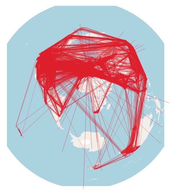
From the images below, you can see the vast number of vectors these freely available datasets contain just for one single day.
You can see in the image that the data is noisy, and must be further cleaned and filtered. Gaps in coverage and recording lead to trajectories spanning the world - and subsequently lead to wrong and misleading results. Nevertheless, we’ll skip this extensive cleansing step today (but might cover this as a separate blog post) and move on with our analysis focusing on a rather small area.
Let’s investigate the trajectories and play through some interesting scenarios.
|
1 2 |
select count(distinct icao24) from flightsegments; |
|
1 2 3 4 5 |
flightanalysis=# select count(distinct icao24) from flightsegments; count ------- 41663 (1 row) |
|
1 2 3 4 5 |
flightanalysis=# select avg(duration(trip)) from flightsegments where st_length(trajectory(trip::tgeogpoint)) > 0; avg ----------------- 03:50:48.245525 (1 row) |
For this kind of analysis, download and import country borders from Natural Earth first.
|
1 2 3 4 5 6 7 8 9 10 |
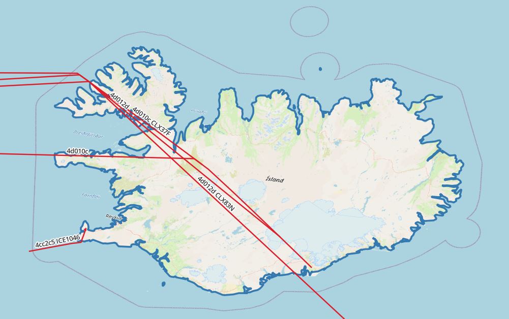
select icao24, callsign, trajectory(atPeriod(T.Trip, '[2022-02-28 00:00:00+00, [2022-2-28 03:00:00+00]'::period)) FROM flightsegments T, ne_10m_admin_0_countries R WHERE T.Trip && stbox(R.geom, '[2022-02-28 00:00:00+00, [2022-02-28 03:00:00+00]'::period) AND st_intersects(trajectory(atPeriod(T.Trip, '[2022-02-28 00:00:00+00, [2022-2-28 03:00:00+00]'::period)), r.geom) and R.name = 'Iceland' and st_length(trajectory(atPeriod(T.Trip, '[2022-02-28 00:00:00+00, [2022-2-28 03:00:00+00]'::period))::geography) > 0 |
|
1 2 3 4 5 6 7 8 9 10 11 12 13 14 15 16 17 18 19 |
select icao24, callsign, (duration( (atgeometry((atPeriod(T.Trip::tgeompoint, '[2022-02-28 00:00:00+00, [2022-02-28 03:00:00+00]'::period)), R.geom))))::varchar, trajectory( atgeometry((atPeriod(T.Trip::tgeompoint, '[2022-02-28 00:00:00+00, [2022-02-28 03:00:00+00]'::period)), R.geom)) FROM flightsegments T, ne_10m_admin_0_countries R WHERE T.Trip && stbox(R.geom, '[2022-02-28 00:00:00+00, [2022-02-28 03:00:00+00]'::period) AND st_intersects(trajectory(atPeriod(T.Trip, '[2022-02-28 00:00:00+00, [2022-2-28 03:00:00+00]'::period)), r.geom) and R.name = 'Iceland' and st_length(trajectory(atPeriod(T.Trip, '[2022-02-28 00:00:00+00, [2022-2-28 03:00:00+00]'::period))::geography) > 0 |
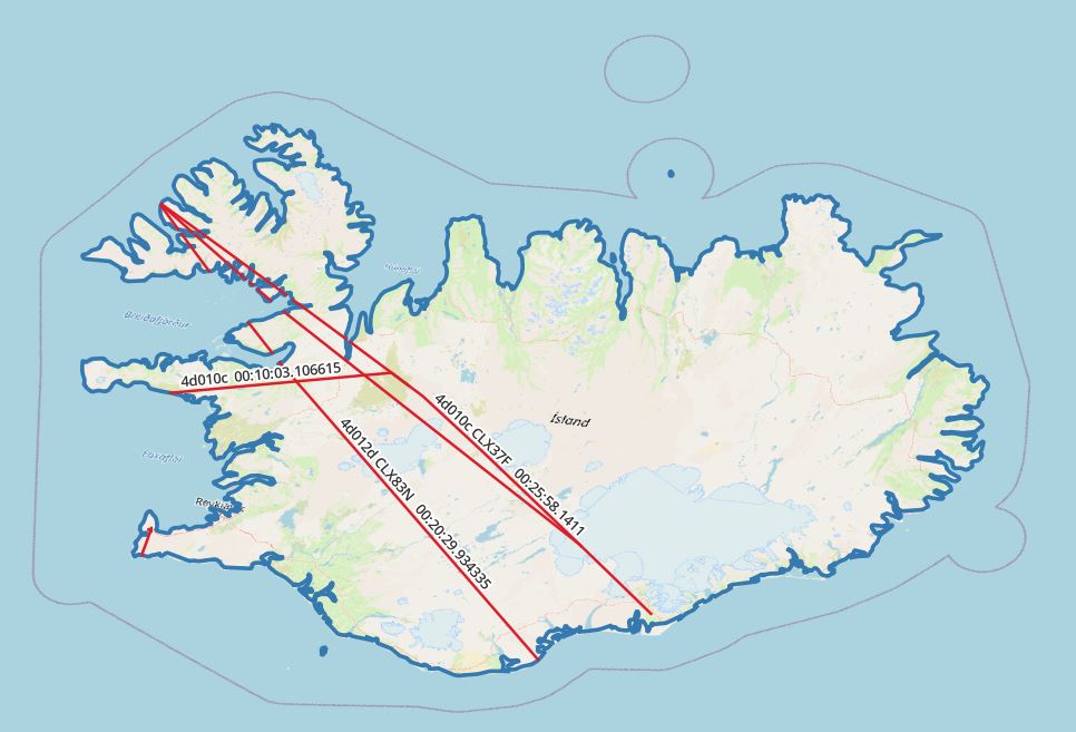
Note that in this case, the plane did not leave the country during this trip.
|
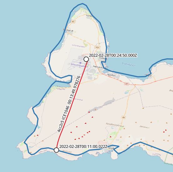
1 2 3 4 5 6 7 8 9 10 11 12 13 14 15 16 17 18 19 20 21 22 23 24 25 26 27 |
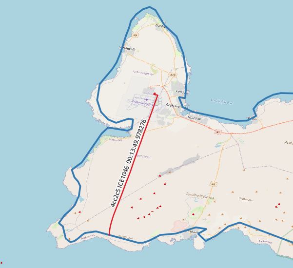
with segments as ( select icao24, callsign, unnest(sequences( atgeometry( (atPeriod(T.Trip::tgeompoint, '[2022-02-28 00:00:00+00, [2022-02-28 03:00:00+00]'::period)), R.geom))) segment FROM flightsegments T, ne_10m_admin_0_countries R WHERE T.Trip && stbox(R.geom, '[2022-02-28 00:00:00+00, [2022-02-28 03:00:00+00]'::period) AND st_intersects(trajectory(atPeriod(T.Trip, '[2022-02-28 00:00:00+00, [2022-2-28 03:00:00+00]'::period)), r.geom) and R.name = 'Iceland' and trim(callsign) = 'ICE1046' and st_length(trajectory(atPeriod(T.Trip, '[2022-02-28 00:00:00+00, [2022-2-28 03:00:00+00]'::period))::geography) > 0) select icao24,callsign, st_startpoint(getvalues(segment)), st_endpoint(getvalues(segment)), starttimestamp(segment), endtimestamp(segment) from segments |
MobilityDB’s rich feature stack drastically simplifies analysis on spatio-temporal data. If I may be allowed to imagine further uses for it, various businesses come to my mind where it could be applied in a smart and efficient manner. Toll systems, surveillance, logistics - just to name a few. Finally, its upcoming release will pave the way for new usages, from research and test utilization to production scenarios.
I hope you enjoyed this session. Learn more about using PostGIS by checking out my blog on spatial datasets based on the OpenStreetMap service
In case you want to learn more about PostGIS and Mobility, just get in touch with the folks from CYBERTEC. Stay tuned!
Missing indexes are a key ingredient if you are looking for a perfect recipe to ruin performance in the most efficient way possible. 🙂 However, if you want to ensure that your database performs well and if you are generally not in favor of user complaints – better watch out for missing indexes and make sure that all relevant tables are properly taken care of. One PostgreSQL index can make all the difference in performance.
To help you understand, I have compiled this little guide about how to locate missing indexes, what you can do to fix them, and how to achieve good database performance.
In order to demonstrate how to find missing indexes, I have to first create a test database. One way to do it is to use pgbench:
|
1 2 3 4 5 6 7 8 9 10 11 12 13 |
[hs@hansmacbook ~]$ pgbench -i -s 100 test dropping old tables... NOTICE: table 'pgbench_accounts' does not exist, skipping NOTICE: table 'pgbench_branches' does not exist, skipping NOTICE: table 'pgbench_history' does not exist, skipping NOTICE: table 'pgbench_tellers' does not exist, skipping creating tables... generating data (client-side)... 10000000 of 10000000 tuples (100%) done (elapsed 13.65 s, remaining 0.00 s) vacuuming... creating primary keys... done in 19.92 s (drop tables 0.00 s, create tables 0.00 s, client-side generate 13.70 s, vacuum 1.95 s, primary keys 4.27 s). |
What happens here is that pgbench just provided us with a little sample database which contains 4 tables.
|
1 2 3 4 5 6 7 8 9 |
test=# d+ List of relations Schema | Name | Type | Owner | Persistence | Access method | Size | Description --------+------------------+-------+-------+-------------+---------------+---------+------------- public | pgbench_accounts | table | hs | permanent | heap | 1281 MB | public | pgbench_branches | table | hs | permanent | heap | 40 kB | public | pgbench_history | table | hs | permanent | heap | 0 bytes | public | pgbench_tellers | table | hs | permanent | heap | 80 kB | (4 rows) |
This database is perfectly indexed by default, so we have to drop some indexes in order to find something we can fix later:
|
1 2 3 4 5 6 7 8 9 10 11 12 13 14 |
test=# d pgbench_accounts Table 'public.pgbench_accounts' Column | Type | Collation | Nullable | Default ----------+---------------+-----------+----------+--------- aid | integer | | not null | bid | integer | | | abalance | integer | | | filler | character(84) | | | Indexes: 'pgbench_accounts_pkey' PRIMARY KEY, btree (aid) test=# ALTER TABLE pgbench_accounts DROP CONSTRAINT pgbench_accounts_pkey; ALTER TABLE |
We have simply dropped the primary key: which is, internally, nothing other than a unique index which does not allow NULL entries.
Before we start running our benchmark to see how bad performance really gets, you need to make sure that the most important tool to handle performance problems is installed and active: pg_stat_statements. Without pg_stat_statements, tracking down performance problems is unnecessarily hard.
Therefore consider performing the next steps to install pg_stat_statements:
Once this is done, we are ready to run our benchmark. Let's see what happens:
|
1 2 3 4 5 6 7 8 9 10 11 12 13 |
[hs@hansmacbook ~]$ pgbench -c 10 -T 60 -j 10 test pgbench (14.1) starting vacuum...end. transaction type: scaling factor: 100 query mode: simple number of clients: 10 number of threads: 10 duration: 60 s number of transactions actually processed: 252 latency average = 2446.148 ms initial connection time = 8.833 ms tps = 4.088061 (without initial connection time) |
Despite opening 10 connections (-c 10) and proving pgbench with 10 threads (-j 10) we managed to run 4 - yes, 4 - transactions per second. One might argue that hardware is the problem, but it's definitely not:
|
1 2 3 4 5 6 |
Model Name: MacBook Pro Model Identifier: MacBookPro16,1 Processor Name: 8-Core Intel Core i9 Processor Speed: 2,3 GHz Number of Processors: 1 Total Number of Cores: 8 |
This is a modern, 8 core machine. Even if the clockspeed were 10 times as high, we would have topped out at 40 transactions per second. That's still way below what you would expect.
The first clue that indexes might be missing can be found in pg_stat_user_tables. The following table contains the relevant columns:
|
1 2 3 4 5 6 7 8 9 10 11 |
test=# d pg_stat_user_tables View 'pg_catalog.pg_stat_user_tables' Column | Type ... ---------------------+---------------- … relid | oid ... schemaname | name ... relname | name ... seq_scan | bigint ... seq_tup_read | bigint ... idx_scan | bigint ... ... |
What we see here is the name of the table (relname) including the schemaname. Then we can see how often our table has been read sequentially (seq_scan) and how often an index has been used (idx_scan). Finally, there is the most relevant information: seq_tup_read. So what does that mean? It actually tells us how many rows the system had to process to satisfy all those sequential scans. This number is really really important and I cannot stress it enough: If “a lot” is read “really often” it will lead to an insane entry in the seq_tup_read column. That also means we have to process an enormous number of rows to read a table sequentially again and again.
|
1 2 3 4 5 6 7 8 9 10 11 12 13 14 15 |
test=# SELECT schemaname, relname, seq_scan, seq_tup_read, idx_scan, seq_tup_read / seq_scan AS avg FROM pg_stat_user_tables WHERE seq_scan > 0 ORDER BY seq_tup_read DESC; schemaname | relname | seq_scan | seq_tup_read | idx_scan | avg ------------+------------------+----------+--------------+----------+--------- public | pgbench_accounts | 954 | 5050000000 | | 5293501 public | pgbench_branches | 254 | 25400 | 0 | 100 public | pgbench_tellers | 1 | 1000 | 252 | 1000 (3 rows) |
This one is true magic. It returns those tables which have been hit by sequential scans the most and tells us how many rows a sequential scan has hit on average. In the case of our top query, a sequential scan has read 5 million rows on average, and indexes were not used at all. This gives us a clear indicator that something is wrong with this table. If you happen to know the application, a simple d will uncover the most obvious problems. However, let us dig deeper and confirm our suspicion:
As stated before, pg_stat_statements is really the gold standard when it comes to finding slow queries. Usually, those tables which show up in pg_stat_user_tables will also rank high in some of the worst queries shown in pg_stat_statements.
The following query can uncover the truth:
|
1 2 3 4 5 6 7 8 9 10 11 12 13 14 15 16 17 18 19 |
test=# SELECT query, total_exec_time, calls, mean_exec_time FROM pg_stat_statements ORDER BY total_exec_time DESC; -[ RECORD 1 ]---+------------------------------------------------------------------- query | UPDATE pgbench_accounts SET abalance = abalance + $1 WHERE aid = $2 total_exec_time | 433708.0210760001 calls | 252 mean_exec_time | 1721.0635756984136 -[ RECORD 2 ]---+------------------------------------------------------------------- query | SELECT abalance FROM pgbench_accounts WHERE aid = $1 total_exec_time | 174819.2974120001 calls | 252 mean_exec_time | 693.7273706825395 … |
Wow, the top query has an average execution time of 1.721 seconds! That is a lot. If we examine the query, we see that there is only a simple WHERE clause which filters on “aid”. If we take a look at the table, we discover that there is no index on “aid” - which is fatal from a performance point of view.
Further examination of the second query will uncover precisely the same problem.
Let's deploy the index and reset pg_stat_statements as well as the normal system statistics created by PostgreSQL:
|
1 2 3 4 5 6 7 8 9 10 11 12 13 14 |
test=# CREATE UNIQUE INDEX idx_accounts ON pgbench_accounts (aid); CREATE INDEX test=# SELECT pg_stat_statements_reset(); pg_stat_statements_reset -------------------------- (1 row) test=# SELECT pg_stat_reset(); pg_stat_reset --------------- (1 row) |
|
1 2 3 4 5 6 7 8 9 10 11 12 13 |
[hs@hansmacbook ~]$ pgbench -c 10 -T 60 -j 10 test pgbench (14.1) starting vacuum...end. transaction type: scaling factor: 100 query mode: simple number of clients: 10 number of threads: 10 duration: 60 s number of transactions actually processed: 713740 latency average = 0.841 ms initial connection time = 7.541 ms tps = 11896.608085 (without initial connection time) |
What an improvement. The database speed has gone up 3000 times. No “better hardware” in the world could provide us with this type of improvement. The takeaway here is that a SINGLE missing PostgreSQL index in a relevant place can ruin the entire database and keep the entire system busy without yielding useful performance.
What is really important to remember is the way we have approached the problem. pg_stat_user_tables is an excellent indicator to help you figure out where to look for problems. Then you can inspect pg_stat_statements and look for the worst queries. Sorting by total_exec_time DESC is the key.
If you want to learn more about PostgreSQL and database performance in general, I can highly recommend Laurenz Albe’s post about “Count(*) made fast” or his post entitled Query Parameter Data Types and Performance.
In order to receive regular updates on important changes in PostgreSQL, subscribe to our newsletter, or follow us on Facebook or LinkedIn.
Range types have been around in PostgreSQL for quite some time and are successfully used by developers to store various kinds of intervals with upper and lower bounds. However, in PostgreSQL 14 a major new feature has been added to the database which makes this feature even more powerful: multiranges. To help you understand multiranges, I have compiled a brief introduction outlining the basic concepts and most important features.
Before we dive into multiranges, I want to quickly introduce basic range types so that you can compare what was previously available with what is available now. Here's a simple example:
|
1 2 3 4 5 |
test=# SELECT int4range(10, 20); int4range ----------- [10,20) (1 row) |
The important thing to note here is that ranges can be formed on the fly. In this case I've created an int4 range. The ranges starts at 10 (which is included) and ends at 20 (which is not included anymore). Basically, every numeric data type that can be sorted can be turned into a range.
What's important to see is that PostgreSQL will ensure that the range is indeed valid which means that the upper bound has to be higher than the lower bound and so on:
|
1 2 |
test=# SELECT int4range(432, 20); ERROR: range lower bound must be less than or equal to range upper bound |
Well, in addition to validation, PostgreSQL provides a rich set of operators. One of the basic operations you'll often need is a way to check whether a value is inside a range or not. Here's how it works:
|
1 2 3 4 5 |
test=# SELECT 17 <@ int4range(10, 20); ?column? ---------- t (1 row) |
You can see from the above that 17 is indeed between 10 and 20 in the table. It's a simple example, but this is also very useful in more complex cases.
It's also possible to use ranges as data types which can be part of a table:
|
1 2 3 4 5 6 7 8 9 |
test=# CREATE TABLE t_range (id serial, t tstzrange); CREATE TABLE test=# INSERT INTO t_range (t) VALUES ('['2022-01-01', '2022-12-31']') RETURNING *; id | t ----+----------------------------------------------------- 1 | ['2022-01-01 00:00:00-05','2022-12-31 00:00:00-05'] (1 row) INSERT 0 1 |
In this case, I've used the tstzrange (“timestamp with time zone range”), and I've successfully inserted a value.
The beauty here is that the operators are available are consistent and work the same way for all range types. This makes them relatively easy to use.
So what are multiranges? The idea is simple: A multirange is a compilation of ranges. Instead of storing just two values, you can store as many pairs as you want. Let 's take a look at a practical example:
|
1 2 3 4 5 |
test=# SELECT int4multirange(int4range(10, 20), int4range(40, 50)); int4multirange ------------------- {[10,20),[40,50)} (1 row) |
In this case, the multirange has been formed on the fly using two ranges. However, you can stuff in as many value pairs as you want:
|
1 2 3 4 5 6 7 8 9 10 |
test=# SELECT int4multirange( int4range(10, 20), int4range(40, 50), int4range(56, 62), int4range(80, 90) ); int4multirange ----------------------------------- {[10,20),[40,50),[56,62),[80,90)} (1 row) |
PostgreSQL has a really nice features which can be seen when ranges are formed. Consider the following example:
|
1 2 3 4 5 6 7 8 9 |
test=# SELECT int4multirange( int4range(10, 20), int4range(12, 25), int4range(38, 42) ); int4multirange ------------------- {[10,25),[38,42)} (1 row) |
As you can see, multiple ranges are folded together to form a set of non-overlapping parts. This happens automatically and greatly reduces complexity.
A multirange can also be used as a data type and stored inside a table just like any other value:
|
1 2 3 4 5 6 7 8 9 10 11 12 13 |
test=# CREATE TABLE t_demo (id int, r int4multirange); CREATE TABLE test=# INSERT INTO t_demo SELECT 1, int4multirange( int4range(10, 20), int4range(12, 25), int4range(38, 42)) RETURNING *; id | r ----+------------------- 1 | {[10,25),[38,42)} (1 row) INSERT 0 1 |
The way you query this type of column is pretty straightforward and works as follows:
|
1 2 3 4 |
test=# SELECT * FROM t_demo WHERE 17 <@ r; id | r ----+------------------- 1 | {[10,25),[38,42)} |
You can simply apply the operator on the column, and you're good to do. In our example, one row is returned which is exactly what we expect.
So far, you've seen that ranges have a beginning and a clearly defined end. However, there is more.
In PostgreSQL, a range is aware of the concept of “infinity”.
Here is an example:
|
1 2 3 4 5 6 |
test=# SELECT numrange(NULL, 10); numrange ---------- (,10) (1 row) |
This range starts with -INFINITY and ends at 10 (not included).
Again, you're able to fold single ranges into a bigger block:
|
1 2 3 4 5 6 7 8 9 10 11 12 13 14 |
test=# SELECT numrange(NULL, 10), numrange(8, NULL); numrange | numrange ----------+---------- (,10) | [8,) (1 row) test=# SELECT nummultirange( numrange(NULL, 10), numrange(8, NULL) ); nummultirange --------------- {(,)} (1 row) |
The example shows a range than spans all numbers (= - INFINITY all the way to +INFINITY). The following query is proof of this fact:
|
1 2 3 4 5 6 7 8 |
test=# SELECT 165.4 <@ nummultirange( numrange(NULL, 10), numrange(8, NULL) ); ?column? ---------- t (1 row) |
The result is true: 165.4 is indeed within the range of valid numbers.
That's not all: you can perform basic operations using these ranges. Now just imagine what it would take to do such calculations by hand in some application. It would be slow, error-prone and in general, pretty cumbersome:
|
1 2 3 4 5 |
test=# SELECT nummultirange(numrange(1, 20)) - nummultirange(numrange(4, 6)); ?column? ---------------- {[1,4),[6,20)} (1 row) |
You can deduct ranges from each other and form a multirange, which represents two ranges and a gap in between. The next example shows how intersections can be calculated:
|
1 2 3 4 5 |
test=# SELECT nummultirange(numrange(1, 20)) * nummultirange(numrange(4, 6)); ?column? ---------- {[4,6)} (1 row) |
There are many more of these kinds of operations you can use to work with ranges. A complete list of all functions and operators is available in the PostgreSQL documentation.
The final topic I want to present is how to aggregate ranges into bigger blocks. Often, data is available in a standard form, and you want to do something fancy with it. Let 's create a table:
|
1 2 3 4 5 6 7 8 9 10 11 |
test=# CREATE TABLE t_holiday (name text, h_start date, h_end date); CREATE TABLE test=# INSERT INTO t_holiday VALUES ('hans', '2020-01-10', '2020-01-15'); INSERT 0 1 test=# INSERT INTO t_holiday VALUES ('hans', '2020-03-04', '2020-03-12'); INSERT 0 1 test=# INSERT INTO t_holiday VALUES ('joe', '2020-01-04', '2020-03-02'); INSERT 0 1 |
I've created a table and added 3 rows. Note that data is stored in the traditional way (“from / to”).
What you can do now is to form ranges on the fly and create a multirange using the range_agg function:
|
1 2 3 4 5 |
test=# SELECT range_agg(daterange(h_start, h_end)) FROM t_holiday; range_agg --------------------------------------------------- {[2020-01-04,2020-03-02),[2020-03-04,2020-03-12)} (1 row) |
What's important here is that you can do more than create a multirange – you can also unnest such a data type and convert it into single entries:
|
1 2 3 4 5 6 7 8 |
test=# SELECT x, lower(x), upper(x) FROM unnest((SELECT range_agg(daterange(h_start, h_end)) FROM t_holiday)) AS x; x | lower | upper -------------------------+------------+------------ [2020-01-04,2020-03-02) | 2020-01-04 | 2020-03-02 [2020-03-04,2020-03-12) | 2020-03-04 | 2020-03-12 (2 rows) |
Let's think about this query: Basically, aggregation and unnesting allow you to answer questions such as: “How many continuous periods of activity did we see?” That can be really useful if you are, for example, running data warehouses.
In general, multiranges are a really valuable extension on top of what PostgreSQL already has to offer. This new feature in PostgreSQL v14 allows us to offload many things to the database which would have otherwise been painful to do and painful to implement on your own.
If you want to learn more about PostgreSQL data types, take a look at Laurenz Albe's recent blog on Query Parameter Data Types and Performance, and if you are interested in data type abstraction check out my blog about CREATE DOMAIN.
Date and time are relevant to pretty much every PostgreSQL application. A new function was added to PostgreSQL 14 to solve a problem which has caused challenges for many users out there over the years: How can we map timestamps to time bins? The function is called date_bin.
What people often do is round a timestamp to a full hour. That's commonly done using the date_trunc function. But what if you want to round data so that it fits into a 30-minute or a 15-minute grid?
Let's take a look at an example:
|
1 2 3 4 5 6 |
test=# SELECT date_bin('30 minutes', '2022-03-04 14:34', '1970-01-01 00:00'); date_bin ------------------------ 2022-03-04 14:30:00+00 (1 row) |
In that case, we want to round for the next half hour: the date_bin function will do the job. The first parameter defines the size of the bins. In our case, it's 30 minutes. The second parameter is the variable we want to round. What's interesting is the third variable. Look at it this way: If we round to a precision of 30 min., what value do we want to start at? Is it 30 min after the full hour, or maybe 35 min? The third value is therefore similar to a baseline where we want to start. In our case, we want to round to 30 min intervals relative to a full hour. Therefore the result is 14:30.
The following parameter sets the baseline to 14:31 and the interval should be 20 min. That's why it comes up with a result of 14:31:
|
1 2 3 4 5 6 |
test=# SELECT date_bin('20 minutes', '2022-03-04 14:49', '1970-01-01 14:31'); date_bin ------------------------ 2022-03-04 14:31:00+00 (1 row) |
If we use a slightly higher value, PostgreSQL will put it into the next time bin:
|
1 2 3 4 5 6 |
test=# SELECT date_bin('20 minutes', '2022-03-04 14:54', '1970-01-01 14:31'); date_bin ------------------------ 2022-03-04 14:51:00+00 (1 row) |
date_bin is super useful, because it gives us a lot of flexibility which can't be achieved using the date_trunc function alone. date_trunc can basically only round to full hours, full days, and so forth.
The date_bin function is adaptable and offers many new features on top of what PostgreSQL already has to offer.
In order to receive regular updates on important changes in PostgreSQL, subscribe to our newsletter, or follow us on Facebook or LinkedIn.