Introduction to Time Series Forecasting

By Kevin Speyer - Time Series Forecast - This post shows you how to approach a time series problem using machine learning techniques. Predicting the behavior of a variable over time is a common problem that one encounters in many industries, from prices of assets on the stock market to the amount of transactions per minute on a server. Despite its importance, time series forecasting is a topic often overlooked in Machine Learning. Moreover, many online courses don't mention the topic at all.

Time series analysis is particularly hard because there is a difficulty that doesn't occur with other problems in Machine Learning: The data has a particular order and it is highly correlated. This means that if you take two observations with the exact same attribute values, the outcome may be totally different due to the recent past measurements.

Implications

This has other practical implications when you attack the problem. For example, you can't split the data between training and validation sets like you would with typical machine learning problems, because the order of the data itself contains a lot of information. One correct way to split the data set in this case would be to keep the first 3/4 of the observations to train the model, and the final 1/4 to validate and test the model's accuracy. There are other more sophisticated ways to split the data, like the rolling window method, that we encourage the reader to look into.

In this case, we'll use the famous ARIMA model to predict the monthly industrial production of electric and gas utilities in the United States from the years 1985–2018. The data can be extracted from the Federal Reserve  or from kaggle.

The ARIMA model

The AutoRegressive Integrated Moving Average (ARIMA) is the go-to model for time series forecasting. In this case we assume that the behavior of the variable can be estimated only from the values that it has taken in the past and there are no external attributes that influence it (other than noise). These cases are known as univariate time series forecasting.

The ARIMA model is actually a combination of three algorithms:

AR: The AutoRegressive models are just linear regression models that fit the present value based on p previous values. The parameter p gives the number of back-steps that will be taken into account to predict the present value.

MA: The Moving Average model proposes that the output is a linear combination of the current and various past values of a random variable. This model assumes that the data is stationary in time, that is, that the average and the variance do not vary on time. The parameter in this case is the number of past values taken into account q

I: "Integrated" refers to the variable that will be fitted. Instead of trying to forecast the value of the observed variable, it is easier to forecast how different the new value will be with respect to the last one. This means using the difference between consecutive steps as the target variable instead of the observable variable itself. In lots of cases, this is an important step, because it will transform the current non-stationary time series into a stationary series. You can go one step further and use the difference of the difference as your target value. If this reminds you of calculus, you are on the right path! The parameter in this case (i) is the number of differentiating to be performed. i=1 means using the discrete derivative as the target variable, i=2 is using the discrete second derivative as the target variable, and so forth.

Exploring the data set

Loading the data:

Typically, we store data in databases, so the first thing we should do is establish a connection and retrieve it. It's easy to do in Python, use the libraries psycopg2 and pandas as follows:

[sourcecode language="bash" wraplines="false" collapse="false"]

import psycopg2
import pandas as pd
db_name = 'energy'
my_user = 'user'
passwd = '*****'
host_url = 'instance_url'
conn = psycopg2.connect(f'host={host_url} dbname={db_name} ' +
f'user={my_user} password={passwd}')
table_name = 'energy_production'
sql_query = f'select * from {table_name}'
df = pd.read_sql_query(sql_query, conn)
[/sourcecode]

The data consists of 397 records with no missing values. We will now split the data into 200 training values, 70 validation values and 127 test values. It is important to always maintain the order of the data, otherwise it will be impossible to perform a coherent forecast.

It's convenient to observe the training and validation data to observe the behavior of the energy production over time:

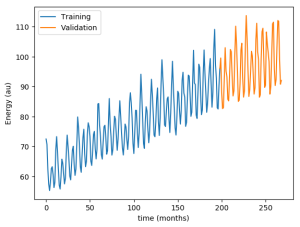
The first thing we can notice from this plot is that the data seems to have different components. On the one hand, the average mean value increases over time. On the other hand, there seems to be a high frequency modulation of energy production.

Fitting the data and forecast

Finally, it's time to adjust the model. We have three hyper-parameters (p, i and d) that we have to choose in order to get the best model possible. A good way to do this is simply to propose some values for the hyperparameters, adjust the model with the training data, and see how well each model performs when predicting the validation data. We call it hyperparameter optimization: don't, as is so often the case, do it wrong:

In hyperparameter optimization, the score of each model with different parameters should be obtained against the validation set, not against the training set.

In Python, this can be done in a couple of lines:

[sourcecode language="bash" wraplines="false" collapse="false"]

n_train = 200
n_valid = 70
n_test = 127

model_par = {}

for ar in [8, 9, 10]:
for ma in [4, 6, 9, 12]:
model_par['ar'] = ar # 9
model_par['i'] = 1  # 1
model_par['ma'] = ma # 4

arr_train = np.array(df.value[0:n_train])
model = ARIMA(arr_train,order=(model_par['ar'],model_par['i'],model_par['ma']))
model_fit = model.fit()
fcst = model_fit.forecast(n_valid)[0]

err = np.linalg.norm(fcst - df.value[n_train:n_train+n_valid]) / n_valid

print(f'err: {err}, parameters: p {model_par['ar']} i:{model_par['i']} q {model_par['ma']}')
[/sourcecode]

The output shows how well the model was able to predict the validation data for each set of parameters:

Here we can observe that the error is minimized by the parameters p=8, i=1 and q=12. Let's see how the forecast looks when compared to the actual data:

[sourcecode language="bash" wraplines="false" collapse="false"]

plt.plot(df.value[:n_train+n_valid-1], label='Data')
plt.plot(range(n_train,n_train+n_valid-1), fcst[:n_valid-1], label= 'Forecast')
#plt.savefig('full_curve.png', bbox_inches='tight',format='png')
plt.xlabel('time (months)')
plt.ylabel('Energy (au)')
plt.legend()
plt.show()

[/sourcecode]

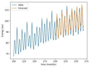
The newly adjusted model predicts the future values of energy prediction pretty well, it looks like we've succeeded!

The problem of predicting the future

Or did we? Now that we have an optimal set of hyperparameters, we should try our model with the test set. Now we take the training and the validation set to adjust our model with p=8, i=1 and q=12, and forecast the values of the test set that it has never seen.

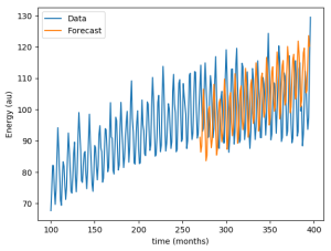
As it turns out, the forecast doesn't fit the data as well as we expected. The mean error went from 0.4 against validation data to 1.1 against test data, almost three times worse! The change in behavior in the data explains this. Energy production ceases to grow, which is something impossible to predict when looking only at the past data. Even for many fully deterministic problems, making predictions far into the future is an impossible task due to highly sensitive initial conditions.

See another of Kevin Speyer's machine learning posts: Series Forecasting with Recurrent Neural Networks (LSTM)