By Kevin Speyer - Hands-on time series forecasting with LSTM - This post will to teach you how to build your first Recurrent Neural Network (RNN) for series predictions. In particular, we are going to use the Long Short Term Memory (LSTM) RNN, which has gained a lot of attention in the last years. LSTM solve the problem of vanishing / exploding gradients in typical RNN. Basically, LSTM have an internal state which is able to remember data over long periods of time, allowing it to outperform typical RNN. There is a lot of material on the web regarding the theory of this network, but there are a lot of misleading articles regarding how to apply this algorithm. In this article we will get straight to the point, building an LSTM network, training it and showing how it is able to make predictions based on the historic data it has seen.
Table of Contents
We will use the data of monthly industrial production of electric and gas utilities in the United States from the years 1985–2018. The data can be extracted from the Federal Reserve or from kaggle. This data has already been used in one of our other posts regarding time series forecasting. First, we will import the packages needed. The LSTM will be constructed with Keras.
[sourcecode language="bash" wraplines="false" collapse="false"]
from __future__ import print_function
import numpy as np
import matplotlib.pyplot as plt
import pandas as pd
from keras.models import Sequential
from keras.layers import Dense, LSTM
[/sourcecode]
If there you get an error here, you should install the packages: Keras, Tensorflow, Pandas, Numpy and Matplotlib. Now, lets read the data from a file, and plot it as a function of time:
[sourcecode language="bash" wraplines="false" collapse="false"]
#Read data
raw_data = pd.read_csv('./Electric_Production_full.csv')
arr_data = np.array(raw_data.Value)
#Plot raw data
plt.plot(arr_data,label = 'Data')
plt.xlabel('time (months)')
plt.ylabel('Energy (au)')
plt.legend()
plt.savefig('data.eps', bbox_inches='tight',format='eps')
plt.show()
[/sourcecode]
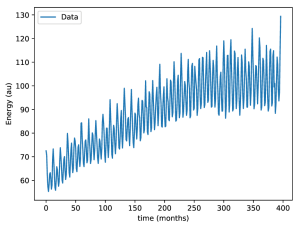
Now, let's define the parameters to use in the script. Of the 397 data points, we will use 270 for training, and the rest for testing. One particularly important parameter is lahead. This is the size of the input that our model will use to predict the next value. In this case we will use lahead = 1, which means that only one point will be used to predict the next value. This seems like an impossible task, given the complex behaviour of the energy as a function of time. The secret is that the LSTM cell has a persistent state that is able to "remember" the data that it has already seen. For a more detailed description, please read the official Keras documentation on LSTM.
[sourcecode language="bash" wraplines="false" collapse="false"]
# Set parameters
n_train = 270
lahead = 1 # time steps that the model incorporates explicitly in the input
# training parameters passed to 'model.fit(...)'
batch_size = 1
epochs = 600
[/sourcecode]
Now let's split the data into training x_train, y_train; and testing x_test, y_test. Please note that y_train is x_train shifted one place, which corresponds to univariable time-series forecasting. This method can be extended for multivariate time analysis. The same is true for x_test and y_test.
[sourcecode language="bash" wraplines="false" collapse="false"]
# Split train and validation
n_data = arr_data.shape[0]
n_valid = n_data - n_train
arr_train = arr_data[:n_train]
arr_valid = arr_data[n_train:]
# split into input and target
x_data = arr_train[:n_train-1]
y_data = arr_train[1:] # same as x_data, but with lag
reshape_3 = lambda x: x.reshape((x.shape[0], 1, 1))
x_train = reshape_3(x_data)
x_test = reshape_3(arr_valid[:-1])
reshape_2 = lambda x: x.reshape((x.shape[0], 1))
y_train = reshape_2(y_data)
y_test = reshape_2(arr_valid[1:])
[/sourcecode]
Let's build a model with one LSTM cell, that has one input and 50 outputs. These 50 outputs will be taken as inputs by one Dense layer, which gives the final 1 dimensional output of the model. Please, note the stateful = True when building the model. This allows us to play with the persistent state of the LSTM cell, otherwise the state will be reset after each call.
[sourcecode language="bash" wraplines="false" collapse="false"]
model = Sequential()
model.add(LSTM(20, input_shape=(lahead, 1), batch_size=batch_size,stateful=True))
model.add(Dense(1))
model.compile(loss='mse', optimizer='adam')
model_stateful = model
[/sourcecode]
Now we are ready to train the model!
[sourcecode language="bash" wraplines="false" collapse="false"]
for i in range(epochs):
print('iteration', i + 1, ' of ', epochs)
model_stateful.fit(x_train, y_train, batch_size=batch_size, epochs=1, validation_data=(x_test, y_test), shuffle=False)
model_stateful.reset_states()
[/sourcecode]
Of course we set the shuffle option to False, because in time series analysis the order should be kept always untouched.
To make predictions with the model, we use the predict function. Remember that the model has been reset, so first we will feed it the training data:
[sourcecode language="bash" wraplines="false" collapse="false"]
#Predict training values
predicted_stateful_train = model_stateful.predict(x_train, batch_size=batch_size)
[/sourcecode]
Now, without resetting the model, we will predict the values in the testing set. To be sure that only one input is being used to make the next time step prediction, we will do it in an explicit fashion:
[sourcecode language="bash" wraplines="false" collapse="false"]
#Predict test values one by one:
pred_test = []
for i in range(x_test.shape[0]):
# Note that only one value x_test[i] is passed as input to the model to make a prediction!
pred_test.append(model_stateful.predict(x_test[i].reshape(1,1,1), batch_size=batch_size))
#Convert list to numpy array
pred_test_1 = np.array(pred_test)
[/sourcecode]
Finally, let's se how the prediction compares with the actual data:
[sourcecode language="bash" wraplines="false" collapse="false"]
#Plot
plt.plot(y_test.reshape(-1),label= 'Data')
plt.plot(pred_test_1.reshape(-1),label= 'Forecast one-by-one')
plt.xlabel('time (months)')
plt.ylabel('Energy (au)')
plt.legend()
plt.show()
[/sourcecode]
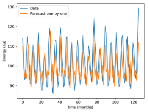
The alignment looks pretty good for a model with one input and such complex behaviour. Now, just to play around a little bit with the stateful model: what happens if we make predictions on the test set, without feeding the training data first? In order to do that, we just need to reset the model, and make predictions directly with the x_test data.
[sourcecode language="bash" wraplines="false" collapse="false"]
model_stateful.reset_states()
# Make predictions after model reset
pred_test_0 = []
for i in range(x_test.shape[0]):
pred_test_0.append(model_stateful.predict(x_test[i].reshape(1,1,1), batch_size=batch_size))
pred_test_0 = np.array(pred_test_0)
plt.plot(y_test.reshape(-1),label= 'Data')
plt.plot(y_test.reshape(-1),label= 'Data')
plt.plot(pred_test_1.reshape(-1),label= 'Forecast')
plt.plot(pred_test_0.reshape(-1),label= 'Forecast reset')
plt.xlabel('time (months)')
plt.ylabel('Energy (au)')
plt.legend()
plt.show()
[/sourcecode]
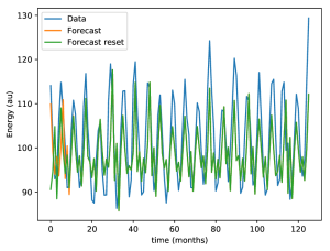
Here is what is happening: the forecast of the reset model (green curve) has a poor performance at the beginning, since it has no previous values to determine the next ones. As the reset model sees mode data, the forecast is on par with the non-reset model (orange) and is able to catch up and make a reasonable forecast compared with the actual data (blue).
+43 (0) 2622 93022-0
office@cybertec.at
You are currently viewing a placeholder content from Facebook. To access the actual content, click the button below. Please note that doing so will share data with third-party providers.
More InformationYou are currently viewing a placeholder content from X. To access the actual content, click the button below. Please note that doing so will share data with third-party providers.
More Information
Leave a Reply