By Kaarel Moppel - Improve transaction latency and consequently performance - The topic of transaction performance is as relevant as ever, in spite of constant hardware improvements, we're quite often asked how to improve in that area. But the truth is that when the most important PostgreSQL configuration parameters are already more or less tuned, it is usually really hard to magically squeeze that extra something out of a setup, without also modifying the schema.

What I've noticed is that a lot of people with performance issues seem to still be using "old" spinning disks. Of course there are a lot of different reasons for that (maybe some long-term server lease contracts or losing support if changing hardware configs). But for cases, in which this is done because there's just way too much data and it would get very expensive, there might be some remedy. Most people don't seem to realize that for OLTP systems there's a huge win, if one can already move the indexes of the busiest tables to SSDs or some other low latency media. So here a quick overview on how to do that with some indicative numbers.

Moving indexes to fast storage - improve transaction latency

The process is quite simple.

1. Install/connect/mount the media. This is probably the hardest part.

2. Create a Postgres tablespace (superuser needed). It would then make sense to also adjust the random_page_cost parameter.

3. Move impactful (lots of columns) or existing indexes to that tablespace. NB! This will result in full locking. Also since 9.4 it's actually possible, to move all indexes to some tablespace with "ALTER INDEX ALL IN TABLESPACE", but this would basically mean a downtime, as everything is locked and then the moving starts. One can do it also in a more controlled/manual way, via "CREATE INDEX CONCURRENTLY ... TABLESPACE ... + RENAME INDEX+ DROP INDEX" or maybe use pg_squeeze/pg_repack extensions that can basically do the same.

4. Optionally it might be a good idea to set this new tablespace as default schema is somewhat static.

Trying to compare HDD vs SDD

To "visualize" the possible performance benefits (there are some for sure), I performed a small and simplistic test, comparing HDD and SDD transaction latencies with a lot of random IO – to really hit the disk a lot, I chose a very small amount of RAM (~5% of dataset fits in shared_buffers/kernel cache), but increased max_wal_size a lot so that we wouldn't stall during the test, giving more predictable latencies. To generate random IO easily, I decided to just create 9 extra indexes on the pgbench schema – and having 10 to 20 indexes on a central OLTP table is also actually quite common. Also to only illustrate HDD vs SDD difference on multi-index update latencies, I removed other activities like WAL logging by using unlogged tables, disabling the background writer and changed the pgbench default transaction so that only the UPDATE part on the single pgbench_accounts table would be executed.

HW info: Google Compute Engine (europe-west-1), 1 vCPU, 1 GB RAM, 100GB Standard persistent disk / SSD persistent disk
Postgres info: PG 10.3, max_wal_size=50GB, checkpoint_timeout=1d, shared_buffers=256MB, bgwriter_lru_maxpages=0
Test script:

The results

And the results were quite surprising actually – almost 38x difference in average update latency on 10 indexes! I somehow thought it will be a bit less, maybe 5-10x...

Disk Type	Latency avg.	Latency Stddev.
HDD	141 ms	158 ms
SSD	3.7 ms	2.5 ms

NB! The test doesn't make any claims at absolute truths – I used separate Google cloud machines (same non-disk specs though), which could have different utilization levels, but to counteract, I limited the transaction rate to a very low 10 TPS not to make it a total throughput test but rather a transaction latency test, so in the end it should at least give some idea on possible performance gains. Also we can see that HDD latencies (at least on shared cloud envs) jump quite a lot on random updates, with "Latency Stddev" being bigger than "Latency avg".

Get the latest information about PostgreSQL performance tuning, right here in our blog spot.

This post will deal with how to speed up analytics and window functions in PostgreSQL. As a professional PostgreSQL support company, we see a lot of SQL performance stuff which is worth sharing. One of those noteworthy things happened this week when I was out on a business trip to Berlin, Germany. This (excellent) customer was making extensive use of window functions and analytics. However, there is always room to speed things up.

“Improving SQL performance” or “how to trick the optimizer”

Most people simply write their SQL code and execute it, assuming that the optimizer will take care of things on its own. While this is usually the case there are still corner cases, where some clever optimization - done by a professional - can give you an edge and better database performance.

How to rearrange window functions for better performance

One way to improve speed is by rearranging window functions in a clever way. Consider the following example:

Our example is pretty simple: All we need is a table containing 5 rows:

Let's take a look at an example:

What we have here is a simple aggregation. For the sake of simplicity I have used array_agg, which simply shows, how our data is aggregated. Of course we could also use min, max, sum, count or any other window function.

Now, let's add a second column to the example:

In this case, there are two columns with two different OVER-clauses. Note that those two aggregations are using different sort orders. One column needs ascending data and one needs descending data.

To understand what is really going on here, we can take a look at the execution plan provided by PostgreSQL:

Sorting the data

First of all, PostgreSQL has to read the data and sort by “id”. This sorted data is fed to the first aggregation, before it is passed on to the next sort step (to sort descending). The second sort passes its output to its window aggregation. Finally, the data is again sorted by id because we want the final output to be ordered by the first column. Overall our data has to be sorted three times, which is not a good thing to do.

Optimizing window functions and avoiding excessive sorting

Sorting data three times is clearly not a good idea. Maybe we can do better. Let us simply swap two columns in the SELECT clause:

Skipping a sorting step

Wow, by making this little change we have actually managed to skip one sorting step. First of all, the data is sorted descending because we need it for the first window function. However, the next column will need data in exactly the same order as the final ORDER BY at the end of the query. PostgreSQL knows that and can already use the sorted input. If you are processing a big data set, this kind of optimization can make a huge difference and speed up your queries tremendously.

At this point PostgreSQL is not able (yet?) to make those adjustments for you so some manual improvements will definitely help. Try to adjust your window functions in a way that columns needing identical sorting are actually next to each other.

Read more about window functions in my post about SQL Trickery: Configuring Window Functions

---

In order to receive regular updates on important changes in PostgreSQL, subscribe to our newsletter, or follow us on Twitter, Facebook, or LinkedIn.

Why vacuum?

Whenever rows in a PostgreSQL table are updated or deleted, dead rows are left behind. VACUUM gets rid of them so that the space can be reused. If a table doesn't get vacuumed, it will get bloated, which wastes disk space and slows down sequential table scans (and – to a smaller extent – index scans).

VACUUM also takes care of freezing table rows so to avoid problems when the transaction ID counter wraps around, but that's a different story.

Normally you don't have to take care of all that, because the autovacuum daemon built into PostgreSQL does it for you. To find out more about enabling and disabling autovacuum, read this post.

Problems with vacuum: bloated tables

In case your tables bloat, the first thing you check is whether autovacuum processed them or not:

If your bloated table does not show up here, n_dead_tup is zero and last_autovacuum is NULL, you might have a problem with the statistics collector.

If the bloated table is right there on top, but last_autovacuum is NULL, you might need to configure autovacuum to be more aggressive so that it finishes the table.

But sometimes the result will look like this:

Here autovacuum ran recently, but it didn't free the dead tuples!

We can verify the problem by running VACUUM (VERBOSE):

Why won't VACUUM remove the dead rows?

VACUUM only removes those row versions (also known as “tuples”) that are not needed any more. A tuple is not needed if the transaction ID of the deleting transaction (as stored in the xmax system column) is older than the oldest transaction still active in the PostgreSQL database. (Or, in the whole cluster for shared tables).

This value (22300 in the VACUUM output above) is called the “xmin horizon”.

There are three things that can hold back this xmin horizon in a PostgreSQL cluster:

1. Long-running transactions and VACUUM:

   You can find those and their xmin value with the following query:

   PgSQL

   SELECT pid, datname, usename, state, backend_xmin, backend_xid FROM pg_stat_activity WHERE backend_xmin IS NOT NULL OR backend_xid IS NOT NULL ORDER BY greatest(age(backend_xmin), age(backend_xid)) DESC;

   1 2 3 4

   SELECT pid, datname, usename, state, backend_xmin, backend_xid FROM pg_stat_activity WHERE backend_xmin IS NOT NULL OR backend_xid IS NOT NULL ORDER BY greatest(age(backend_xmin), age(backend_xid)) DESC;

   You can use the pg_terminate_backend() function to terminate the database session that is blocking your VACUUM.

    

2. Abandoned replication slots and VACUUM:

   A replication slot is a data structure that keeps the PostgreSQL server from discarding information that is still needed by a standby server to catch up with the primary.

   If replication is delayed or the standby server is down, the replication slot will prevent VACUUM from deleting old rows.

   You can find all replication slots and their xmin value with this query:

   PgSQL

   SELECT slot_name, slot_type, database, xmin FROM pg_replication_slots ORDER BY age(xmin) DESC;

   1 2 3

   SELECT slot_name, slot_type, database, xmin FROM pg_replication_slots ORDER BY age(xmin) DESC;

   Use the pg_drop_replication_slot() function to drop replication slots that are no longer needed.

   Note: This can only happen with physical replication if hot_standby_feedback = on. For logical replication there is a similar hazard, but only it only affects system catalogs. Examine the column catalog_xmin in that case.

    

3. Orphaned prepared transactions and VACUUM:

   During two-phase commit, a distributed transaction is first prepared with the PREPARE statement and then committed with the COMMIT PREPARED statement.

   Once Postgres prepares a transaction, the transaction is kept “hanging around” until it Postgres commits it or aborts it. It even has to survive a server restart! Normally, transactions don't remain in the prepared state for long, but sometimes things go wrong and the administrator has to remove a prepared transaction manually.

   You can find all prepared transactions and their xmin value with the following query:

   PgSQL

   SELECT gid, prepared, owner, database, transaction AS xmin FROM pg_prepared_xacts ORDER BY age(transaction) DESC;

   1 2 3

   SELECT gid, prepared, owner, database, transaction AS xmin FROM pg_prepared_xacts ORDER BY age(transaction) DESC;

   Use the ROLLBACK PREPARED SQL statement to remove prepared transactions.

    

4. Standby server with hot_standby_feedback = on and VACUUM:

   Normally, the primary server in a streaming replication setup does not care about queries running on the standby server. Thus, VACUUM will happily remove dead rows which may still be needed by a long-running query on the standby, which can lead to replication conflicts. To reduce replication conflicts, you can set hot_standby_feedback = on on the standby server. Then the standby will keep the primary informed about the oldest open transaction, and VACUUM on the primary will not remove old row versions still needed on the standby.

   To find out the xmin of all standby servers, you can run the following query on the primary server:

   PgSQL

   SELECT application_name, client_addr, backend_xmin FROM pg_stat_replication ORDER BY age(backend_xmin) DESC;

   1 2 3

   SELECT application_name, client_addr, backend_xmin FROM pg_stat_replication ORDER BY age(backend_xmin) DESC;

Read more about PostgreSQL table bloat and autocommit in my post here.

What does PostgreSQL Full-Text-Search have to do with VACUUM? Many readers might actually be surprised that there might be a relevant connection worth talking about at all. However, those two topics are more closely related, than people might actually think. The reason is buried deep inside the code and many people might not be aware of those issues. Therefore I've decided to shed some light on this topic and explain, what is really going on here. The goal is to help end users to speed up their Full-Text-Indexing (FTI) and offer better performance to everybody making use of PostgreSQL.

Controlling VACUUM and autovacuum

Before digging into the real stuff, it is necessary to create some test data. For that purpose, I created a table. Note that I turned autovacuum off so that all operations are fully under my control. This makes it easier to demonstrate, what is going on in PostgreSQL.

In the next step we can create 2 million random texts. For the sake of simplicity, I did not import a real data set containing real texts but simply created a set of md5 hashes, which are absolutely good enough for the job:

Here is what our data looks like:

To make things more efficient, I decided to use the tsvector data type in the table directly. The advantage is that we can directly create a full text index (FTI) on the column:

In PostgreSQL, a GIN index is usually used to take care of “full text search” (FTS).

Finally we run VACUUM to create all those hint bits and make PostgreSQL calculate optimizer statistics.

How GIN indexes work in PostgreSQL

To understand what VACUUM and Full Text Search (FTS) have to do with each other, we first got to see, how GIN indexes actually work: A GIN index is basically a “normal tree” down to the word level. So you can just binary search to find a word easily. However: In contrast to a btree, GIN has a “posting tree” below the word level. So each word only shows up once in the index but points to a potentially large list of entries. For full text search this makes sense because the number of distinct words is limited in real life while a single word might actually show up thousands of times.

The following image shows, what a GIN index looks like:

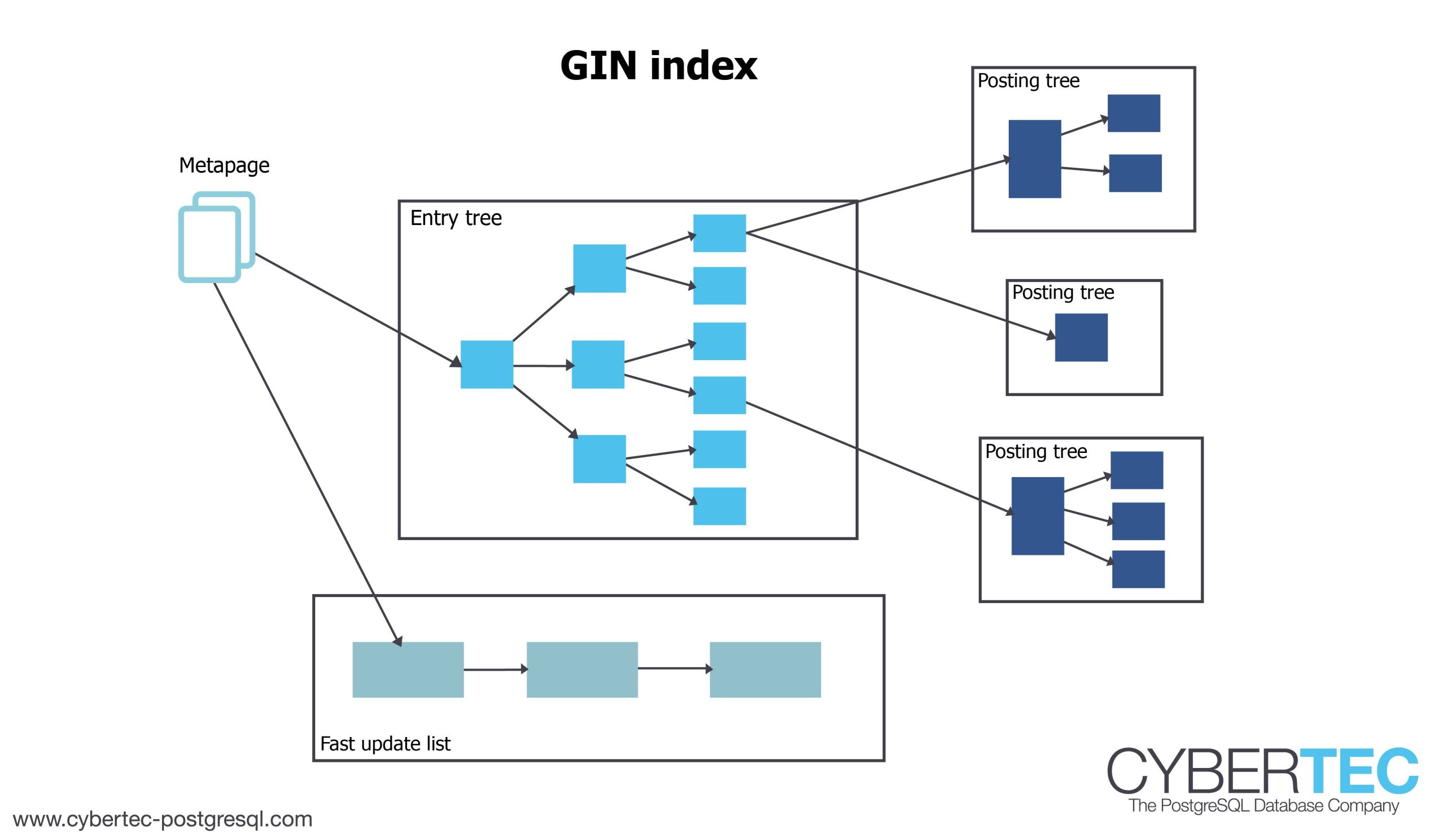
Let us take a closer look at the posting tree itself: It has one entry for pointer to the underlying table. To make it efficient, the posting tree is sorted. The trouble now is: If you insert into the table, changing the GIN index for each row is pretty expensive. Modifying the posting tree does not come for free. Remember: You have to maintain the right order in your posting tree so changing things comes with some serious overhead.

Fortunately there is a solution to the problem: The “GIN pending list”. When a row is added, it does not go to the main index directly. But instead it is added to a “TODO” list, which is then processed by VACUUM. So after a row is inserted, the index is not really in its final state. What does that mean? It means that when you scan the index, you have to scan the tree AND sequentially read what is still in the pending list. In other words: If the pending list is long, this will have some impact on performance. In many cases it can therefore make sense to vacuum a table used to full text search more aggressively as usual. Remember: VACUUM will process all the entries in the pending list.

Measuring the performance impact of VACUUM

To see what is going on behind the scenes, install pgstattuple:

With pgstattuple you can take a look at the internals of the index:

In this case the pending list is empty. In addition to that the index is also pretty small:

Keep in mind: We had 2 million entries and the index is still close to nothing compared to the size of the table:

Let us run a simple query now. We are looking for a word, which does not exist. Note that the query needs ways less than 1 millisecond:

I would also like to point you to something else: “shared hit = 5”. The query only needed 5 blocks of data to run. This is really really good because even if the query has to go to disk, it will still return within a reasonable amount of time.

Let us add more data. Note that autovacuum is off so there are no hidden operations going on:

The same query, which performanced so nicely before, is now a lot slower:

PostgreSQL needs more than 9 milliseconds to run the query. The reason is that there are many pending tuples in the pending list. Also: The query had to access 331 pages in this case, which is A LOT more than before. The GIN pending list reveals the underlying problem:

5 pages + 326 pages = 331 pages. The pending list explains all the additional use of data pages instantly.

Running VACUUM to speed up Full-Text-Search (FTS) in PostgreSQL

Moving those pending entries to the real index is simple. We simply run VACUUM ANALYZE again:

As you can see the pending list is now empty:

The important part is that the query is also a lot slower again because the number of blocks has decreased again.

I think those examples show pretty conclusively that VACUUM does have a serious impact on the performance of your full text indexing. Of course this is only true if a significant part of your data is changed on a regular basis.

The COPY command in PostgreSQL is a simple way to copy data between a file and a table. COPY can either copy the content of a table to or from a table. Traditionally data was copied between PostgreSQL and a file. However, recently a pretty cool feature was added to PostgreSQL: It is now possible to send data directly to the UNIX pipe.

COPY … TO PROGRAM: Sending data to the pipe

The ability to send data directly to the UNIX pipe (or Linux command line) can be pretty useful. You might want to compress your data or change the format on the fly. The beauty of the UNIX shell is that it allows you all kinds of trickery.

If you want to send data to an external program – here is how it works:

In this case, the output of the query is sent to gzip, which compresses the data coming from PostgreSQL and stores the output in a file. As you can see, this is pretty easy and really straight forward.

Copying data between PostgreSQL and other machines

However, in some cases users might desire to store data on some other machine. Note that the program is executed on the database server and not on the client. It is also important to note that only superusers can run COPY … TO PROGRAM. Otherwise people would face tremendous security problems, which is not desirable at all.

Once in a while ,people might not want to store the data exported from the database on the server but send the result to some other host. In this case SSH comes to the rescue. SSH offers an easy way to move data.

Here is an example:

In this case “Lots of data” will be copied over SSH and stored in /directory/big.txt.

The beauty is that we can apply the same technique to PostgreSQL:

To make this work in real life, you have to make sure that SSH keys are in place and ready to use. Otherwise the system will prompt for a password, which is of course not desirable at all. Also keep in mind that the SSH command is executed as “postgres” user (in case your OS user is called “postgres” too).