By Kaarel Moppel

Version 12 of PostgreSQL is not exactly fresh out of the oven, as the first minor release was already announced. However, I think it’s fair to say that this version can be still considered fresh for most users, and surely only a small percentage of users has upgraded. So I think it makes sense to go over some new features. This will be my last article beating on the v12 drum though, I promise 🙂

As usual, there have already been quite a few articles on the planet.postgresql.org feed on that topic, so I’ll try to cover things from another angle and not only concentrate on the main features of PostgreSQL version 12. In general, though, this release was more of an “infrastructure” release, and maybe not so exciting as v11 when it comes to cool new features (with some exceptions)-- however, do take a look as there are hundreds of small changes in every release, so I’m sure you’ll discover something new for yourself. Full release notes can be found here - https://www.postgresql.org/docs/12/release-12.html

“Automatic” performance improvements

Although on average, this release might not be the fastest one, due to some infrastructure changes which also provide other benefits, there are some areas where you’ll see huge performance boosts out of the box, without having to do anything:

Automatic inlining of common table expressions (CTEs)

 This should provide a performance boost for 99% of use cases – and for those rare exceptions where you don’t want to benefit from filter pushdowns and index scans, (for example, in the rare cases where extreme bloat or planner row count misjudgements are a problem) you can override it with the “ MATERIALIZED” keyword, e.g.:

Allow parallelized queries when in SERIALIZABLE isolation mode

Serializable isolation mode is quite rare in the wild due to the resulting performance penalties, but technically, it is the simplest way to fix crappy applications, not taking all parallel activities properly into account - and now it has been much improved for larger amounts of data! Note that for low CPU machines, I usually recommend increasing the default parallelization thresholds (min_parallel_index_scan_size / min_parallel_table_scan_size) a bit. The reason is that both creating the OS processes and syncing incur costs, and it could actually be slower in the end for smallish datasets.

Enable Just-in-Time (JIT) compilation by default

Introduced in v11, this was the optional “killer feature” for those implementing Data Warehouses on Postgres, with up to 50% boosts. Since there were no big problems found with its quite complex functionality, it’s now enabled by default and also kicks in a bit more often. A disclaimer seen at this year’s pgConf.EU though – in some rare cases, for very complex queries, the JIT code generation + optimized execution can take more time than the plain non-optimal execution! Luckily, it’s a “user”-level feature, and can be disabled per session / transaction. Alternatively, you could also tune the “jitting” threshold family of parameters (jit_*_cost), so that small / medium datasets won’t use them.

My favourite developer changes

Support for the SQL/JSON path language

Like the section title says, this feature is an implementation of the SQL standard and allows easy selection and filtering of specific elements of JSON objects, for example, in order to create joins in a more standard fashion. Huge amounts of new structures / functions are now available, by the way, so only the most basic sample is shown below. For more info, check the docs - https://www.postgresql.org/docs/12/functions-json.html#FUNCTIONS-SQLJSON-PATH

Allow foreign keys to reference partitioned tables

With this feature, as of v12, the partitioning functionalities of PostgreSQL could be called complete. There’s a small gotcha with this FK functionality though, limiting its usefulness in some cases: the column being referenced must be a part of the partitioning key! Sadly, this does not play too nice with typical date-based partitioning scenarios, so you’ll need to resort to the usual hacks, like custom validation triggers, or regularly running some FK checking scripts.

Add partition introspection functions

The new pg_partition_root(), pg_partition_ancestors() and pg_partition_tree() functions do what they sound like (well, the pg_partition_tree() doesn’t visualize a real tree, but just a table) and are a real boon, especially for those who are doing multi-level partitioning.

Add connection parameter tcp_user_timeout to control libpq's TCP timeout

Not something for everyone, but it’s a useful new way to signal from the client side that you’re on a bad network, or there’s some overly-aggressive firewall somewhere in between; you will want to de-allocate session resources as soon as possible, if something has gone sour. There are also some server-side “keepalive” params dealing with the same topic but not exactly the same thing; those parameters are for idle connections, and things are measured in seconds there, not in milliseconds.

Show the manual page URL in psql's “h[elp]” output for a SQL command

This is perfect for beginners who might need a bit more background information on some commands, as the default “help” is quite terse (on purpose, of course!). Especially cheering – the feature was added based on my suggestion / complaint 🙂 Thanks guys, you’re awesome!

Allow VACUUM to skip index cleanup

As per the documentation - disabling index cleanup can speed up VACUUM significantly (the more indexes you have, the more noticeable it is) – so it’s perfect for cases where you need to quickly roll out some schema changes and are willing to accept the penalty of more bloated indexes if there’s a lot of simultaneous UPDATE activity.

Add EXPLAIN option SETTINGS to output non-default optimizer settings

This is a nice addition for those urgent troubleshooting cases where it’s easy to miss the obvious, due to some mental pressure. The Git log entry says it all: Query planning is affected by a number of configuration options, and it may be crucial to know which of those options were set to non-default values. With this patch, you can say EXPLAIN (SETTINGS ON) to include that information in the query plan. Only those options which affect planning and contain values different from the built-in default are printed.

Allow logging of statements from only a percentage of transactions

The new “log_transaction_sample_rate” does the above. It’s great for those troubleshooting cases where you want to get real, executable, SQL samples from logs (pg_stat_statements already works with parameterized statements) but don’t want to negatively affect the performance or fill the logs. By the way, if you’re stuck on some lower Postgres version and can’t upgrade in the near future – try the “auto_explain” extension’s “sample_rate” for effectively the same functionality (with some more verbose EXPLAIN output though) as weirdly enough, it has already been there for years.

My favourite DBA changes

Cause recovery to advance to the latest timeline by default

Finally! The previous default’s recovery_target_timeline setting of “current” was a major stumbling stone for beginners making use of PostgreSQL’s “cascading replication” feature and caused quite a few support inquiries for me over the years. It now defaults to “latest,” as it should be.

Parallel automatic index rebuilding

REINDEX CONCURRENTLY was one of the “headline” features of the v12 release, a well-deserved honor: similar behaviour previously required quite a lot of scripting and was thus very tedious and also somewhat dangerous (non-critically).

 The “pg_checksums” utility can now enable/disable page checksums for an offline cluster

PostgreSQL-side checksums serve as an “early warning” system for detecting silent data corruption (only for the blocks being touched, though) and should actually almost always be enabled . Previously, once missed on initialization, it could not be fixed later on. Well, only via dump / reload or upgrading via logical replication...which might not always be desirable or doable. So, this is a very welcome addition.

How big of a downtime are we talking about here? Not too much – for example, for my 64 GB test instance, it took 5 minutes. But I think there are some plans to improve it further to support “live” transitions. And making the process parallel would also of course help, currently it seems to be single threaded, as it could deplete neither my CPU nor the IO subsystem of my SSD. For the “live” scenario it wouldn’t matter too much, though. It would also be nice if the utility could handle some older Postgres versions - when I tried it, it bailed with “error: pg_control CRC value is incorrect” for v11 for example. Well, we can’t have it all, I guess.

Allow CREATE TABLE's tablespace specification for a partitioned table to affect the tablespace of its children

Previously, you had to rely solely on the correct usage of the “default_tablespace” parameter, so this feature will make the DBA’s life a lot easier, once you’re at a scale where you really need some tablespace management. For the “transitioning” Oracle DBA’s – you don’t need or want any extra tablespaces “just for fun” in PostgreSQL, it will only make your life more complex than needed.

Allow values produced by queries to be assigned to pgbench variables

This is one of my favourite ones, me being a huge user of pgbench in general. So what does it allow me to do? For example, it allows me to quickly simulate some locking scenarios, by using only a subset of pgbench-generated accounts, or to force some kind of ordering to account updates. The pgbench scripting language command for this is “gset” and the code would look something like the below:

Allow fractional input for integer server parameters

For example, SET work_mem = '1.5GB' is now allowed. Small code change, but a lot of convenience.

Allow vacuumdb to select tables for vacuum based on their wraparound horizon

This could be a real lifesaver for huge databases where Autovacuum was kept unchecked for a long period of time, and the wraparound horizon is nearing (WARNING messages will pop up in the logs modified) and some quick manual reaction is needed to avoid effective downtime.

One more note

To finish up, I’ll repeat what it says in the release notes, and also mention the huge breaking change in replication management, in case you’ve managed to forget – “recovery.conf” files are dead, gone, history! And the related settings now reside in the main server conf (postgresql.conf / postgresql.auto.conf). This means updating your replication scripts if you’re not using any 3rd party utilities to take care of that, but on the upside - less files, and it’s now possible to inspect those settings from within Postgres sessions.

Hope you found something new and useful here!

 

If you thought that the B-tree index is a technology that was perfected in the 1980s, you are mostly right. But there is still room for improvement, so PostgreSQL v12 (in the tradition of v11) has added some new features in this field. Thanks, Peter Geoghegan!

In this article, I want to explain some of these improvements with examples.

A B-tree index test case

To demonstrate the changes, I'll create an example table on both PostgreSQL v11 and v12:

Tables like this are typically used to implement many-to-many relationships between other tables (entities).

The primary key creates a unique composite B-tree index on the table. The table serves two purposes:

• it ensures that there is at most one entry for each combination of aid and bid
• it can speed up searches for all bids related to a given aid

The second index speeds up searches for all aids related to a given bid.

Adding test data

Now let's insert some rows in ascending numeric order, as is common for artificially generated keys:

Here each bid is related to 10000 aids.

B-tree index improvement 1: INSERT into indexes with many duplicates

The first difference becomes obvious when we compare the size of the index on bid:

In PostgreSQL v11:

In PostgreSQL v12:

The index is 33% bigger in v11.

Explanation

Every bid occurs 10000 times in the index, therefore there will be many leaf pages where all keys are the same (each leaf page can contain a couple of hundred entries).

 

Before v12

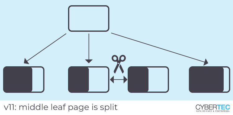
Before v12, PostgreSQL would store such entries in no special order in the index. So if a leaf page had to be split, it was sometimes the rightmost leaf page, but sometimes not. The rightmost leaf page was always split towards the right end to optimize for monotonically increasing inserts. In contrast to this, other leaf pages were split in the middle, which wasted space.

Since v12

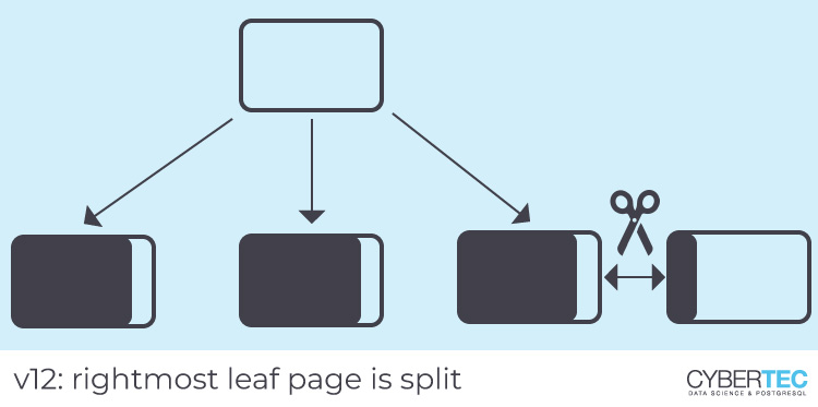
Starting with v12, the physical address (“tuple ID” or TID) of the table row is part of the index key, so duplicate index entries are stored in table order. This will cause index scans for such entries to access the table in physical order, which can be a significant performance benefit, particularly on spinning disks. In other words, the correlation for duplicate index entries will be perfect. Moreover, pages that consist only of duplicates will be split at the right end, resulting in a densely packed index (that is what we observed above).

A similar optimization was added for multi-column indexes, but it does not apply to our primary key index, because the duplicates are not in the first column. The primary key index is densely packed in both v11 and v12, because the first column is monotonically increasing, so leaf page splits occur always at the rightmost page. As mentioned above, PostgreSQL already had an optimization for that.

B-tree index improvement 2: compressed storage of internal index pages

The improvements for the primary key index are not as obvious, since they are almost equal in size in v11 and v12. We will have to dig deeper here.

First, observe the small difference in an index-only scan in both v11 and v12 (repeat the statement until the blocks are in cache):

In PostgreSQL v11:

In PostgreSQL v12:

In v12, one less (index) block is read, which means that the index has one level less. Since the size of the indexes is almost identical, that must mean that the internal pages can fit more index entries. In v12, the index has a greater fan-out.

Explanation

As described above, PostgreSQL v12 introduced the TID as part of the index key, which would waste an inordinate amount of space in internal index pages. So the same commit introduced truncation of “redundant” index attributes from internal pages. The TID is redundant, as are non-key attributes from an INCLUDE clause (these were also removed from internal index pages in v11). But PostgreSQL v12 can also truncate those index attributes that are not needed for table row identification.

In our primary key index, bid is a redundant column and is truncated from internal index pages, which saves 8 bytes of space per index entry. Let's have a look at an internal index page with the pageinspect extension:

In PostgreSQL v11:

In the data entry we see the bytes from aid and bid. The experiment was conducted on a little-endian machine, so the numbers in row 6 would be 0x09C3E5 and 0x3F or (as decimal numbers) 639973 and 63. Each index entry is 24 bytes wide, of which 8 bytes are the tuple header.

In PostgreSQL v12:

The data contain only aid, since bid has been truncated away. This reduces the index entry size to 16, so that more entries fit on an index page.

Upgrade considerations

Since index storage has been changed in v12, a new B-tree index version 4 has been introduced.

Since upgrading with pg_upgrade does not change the data files, indexes will still be in version 3 after an upgrade. PostgreSQL v12 can use these indexes, but the above optimizations will not be available. You need to REINDEX an index to upgrade it to version 4 (this has been made easier with REINDEX CONCURRENTLY in PostgreSQL v12).

Other B-tree index features introduced in v12

There were some other improvements added in PostgreSQL v12. I won't discuss them in detail, but here is a list:

• Reduce locking overhead for B-tree index inserts for improved performance.
• Introduce REINDEX CONCURRENTLY to make it easier to rebuild an index without down-time.
• Improve performance for index-only scans on indexes with many attributes.
• Add a view pg_stat_progress_create_index to report progress for CREATE INDEX and REINDEX.

Conclusion

B-tree indexes have become smarter again in PostgreSQL v12, particularly for indexes with many duplicate entries. To fully benefit, you either have to upgrade with dump/restore or you have to REINDEX indexes after pg_upgrade.

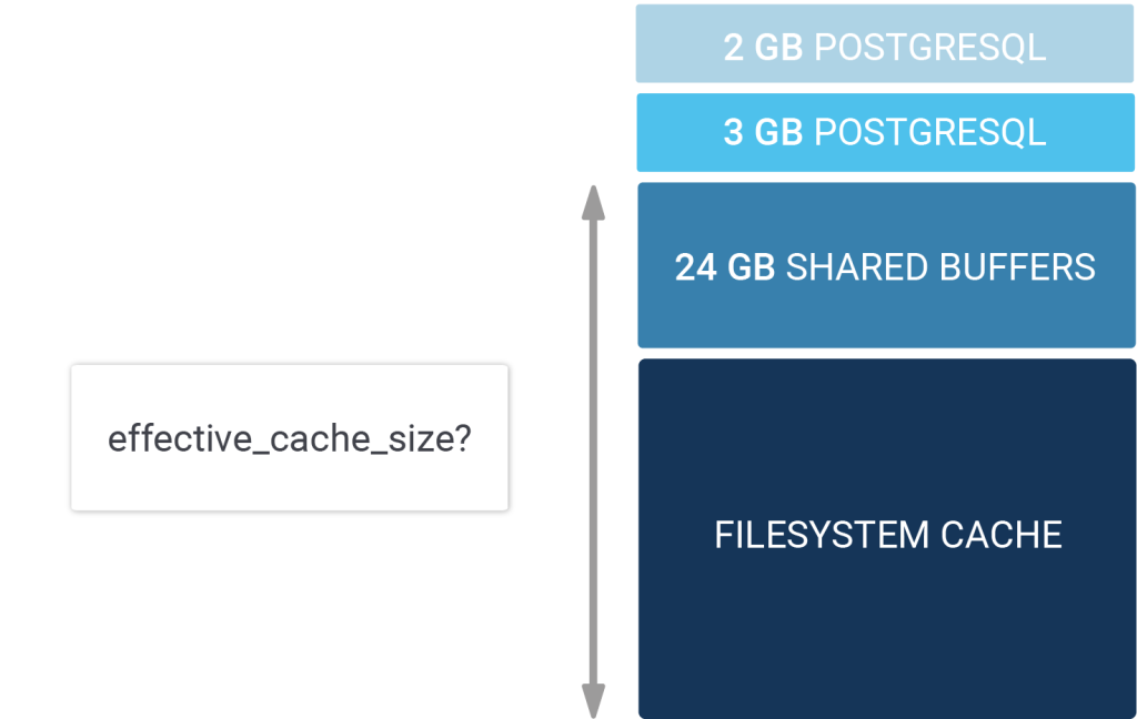
Many PostgreSQL database users might have stumbled over the effective_cache_size parameter in postgresql.conf. But how can it be used to effectively tune the database and how can we speed up PostgreSQL using effective_cache_size? This blog will hopefully answer some of my readers' questions and reveal the hidden power of this secretive setting.

RAM, Linux, PostgreSQL

A lot has been written about RAM, PostgreSQL, and operating systems (especially Linux) over the years. However, to many memory usage is still a mystery and it makes sense to think about it when running a production database system. Let's take a look at a simple scenario and see how memory might be used on a modern server. For the sake of simplicity, let's assume that our server (or VM - virtual machine, ed.) provides us with 100 GB of RAM. 2 GB might be taken by the operating system including maybe some cron jobs, monitoring processes and so on. Then you might have assigned 20 GB of memory to PostgreSQL in the form of shared buffers (=PostgreSQL's I/O cache). In total PostgreSQL might need 25 GB of memory to run in this case. On top of those 20 GB it will take some memory to sort data, keep database connections around and keep some other vital information in mapped memory.

The question is now: What happens to the remaining 73 GB of RAM? The answer is: Some of it might be "free" and available but most of it will end up as  filesystem cache. Whenever Linux does I/O and in case enough free memory is around the filesystem cache will kick in and try to cache the data to avoid disk I/O if possible. The filesystem is vital and can be changed in size dynamically as needed. If PostgreSQL needs more RAM to, say, sort data, it will allocate memory which in turn makes the operating system shrink the filesystem cache as needed to ensure efficiency.

RAM and the PostgreSQL optimizer

The PostgreSQL optimizer is in charge of making sure that your queries are executed in the most efficient way possible. However, to do that it makes sense to know how much RAM there is really around. The system knows about the size if its own memory (= shared_buffers) but what about the filesystem cache? What about your RAID controller and so on? Wouldn't it be cool if you the optimizer knew about all those ressources?

That is exactly what effective_cache_size is all about. It helps the planner to determine how much cache there really is and helps to adjust the I/O cache. Actually,
the explanation I am giving here is already longer than the actual C code in the server. Let's take a look at costsize.c and see what the comment says there:

This code snippet taken directly from costsize.c in the core is basically the only place in the optimizer which takes effective_cache_size into account. As you can see, the formula is only used to estimate the costs of indexes. In short: If PostgreSQL knows that a lot of RAM is around, it can safely assume that fewer pages have to come from disk and more data will come from the cache, which allows the optimizer to make indexes cheaper (relativ to a sequential scan). You will notice that this effect can only be observed if your database is sufficiently large. On fairly small databases you will not observe any changes in execution plans.

effective_cache_size and Gist index creation

However, the PostgreSQL query optimizer is not the only place that checks effective_cache_size. Gist index creation will also check the parameter and
adjust its index creation strategy. The idea is to come up with the buffering strategy during index creation.

Finally ...

If you want to learn more about PostgreSQL memory parameters you can find out more in our post about about work_mem and sort performance.

 

OSM to PostGIS – The Basics

Ever wondered how to import OSM (OpenStreetMap) data into PostGIS [1] for the purpose of visualization and further analytics? Here are the basic steps to do so.
There are a bunch of tools on the market— osm2pgsql; imposm; ogr2org; just to mention some of those. In this article I will focus on osm2pgsql [2] .

Let’s start with the software prerequisites. PostGIS comes as a PostgreSQL database extension, which must be installed in addition to the core database. Up till now, the latest PostGIS version is 3, which was released some days ago. For the current tasks I utilized PostGIS 2.5 on top of PostgreSQL 11.
This brings me to the basic requirements for the import – PostgreSQL >= 9.4 and PostGIS 2.2 are required, even though I recommend installing PostGIS >=2.5 on your database;  it’s supported from 9.4 upwards. Please consult PostGIS’ overall compatibility and support matrix [3] to find a matching pair of components.

Osm2pgsql Setup

Let’s start by setting up osm2pgsql on the OS of your choice – I stick to Ubuntu 18.04.04 Bionic Beaver and compiled osm2gsql from source to get the latest updates.

Install required libraries

sudo apt-get install make cmake g++ libboost-dev libboost-system-dev
libboost-filesystem-dev libexpat1-dev zlib1g-dev
libbz2-dev libpq-dev libproj-dev lua5.2 liblua5.2-dev

Grab the repo

git clone https://github.com/openstreetmap/osm2pgsql.git

Compile

mkdir build && cd build
cmake ..
make
sudo make install

If everything went fine, I suggest checking the resulting binary and its release by executing

./osm2pgsql-version

Data acquisition

In the world of OSM, data acquisition is a topic of its own, and worth writing a separate post discussing different acquisition strategies depending on business needs, spatial extent and update frequency. I won’t get into details here, instead, I’ll just grab my osm data for my preferred area directly from Geofabrik, a company offering data extracts and related daily updates for various regions of the world. This can be very handy when you are just interested in a subregion and therefore don’t want to deal with splitting the whole planet osm depending on your area of interest - even though osm2pgsql offers the possibility to hand over a bounding box as a spatial mask.
As a side note – osm data’s features are delivered as lon/lat by default.

So let’s get your hands dirty and fetch a pbf of your preferred area from Geofabrik’s download servers [4] [5]. For a quick start, I recommend downloading a dataset covering a small area:

wget https://download.geofabrik.de/europe/iceland-latest.osm.pbf

Optionally utilize osmium to check the pbf file by reading its metadata afterwards.

./osm2pgsql-version

Database setup

Before finally importing the osm into PostGIS, we have to set up a database enabling the PostGIS extension. As easy as it sounds – connect to your database with your preferred database client or pgsql, and enable the extension by executing

create extension postgis

Subsequently, execute

select POSTGIS_VERSION()

to validate the PostGIS installation within your database.

Database import

osm2pgsql is a powerful tool to import osmdata into PostGIS offering various parameters to tune. It’s worthwhile to mention the existence of the default-style parameter [6], which defines how osm data is parsed and finally represented in the database. The diagram below shows the common database model generated by osm2pgsql using the default style.

It’s hard to give a recommendation on how this style should be adopted, as this heavily depends on its application. As a rule of thumb, the default style is a good starting point for spatial analysis, visualizations and can even be fed with spatial services, since this layout is supported by various solutions (e.g. Mapnik rendering engine).

I will start off with some basic import routines and then move to more advanced ones. To speed up the process in general, I advise you to define the number of processes and cache in MB to use. Even if this blogpost is not intended as a performance report, I attached some execution times and further numbers for the given parametrized commands to better understand the impact the mentioned parameters have.

The imports were performed on a virtualized Ubuntu 18.04 (KVM) machine equipped with 24 cores (out of 32 logical cores provided by an AMD Ryzen Threadripper 2950X), 24GB RAM, and a dedicated 2TB NVMe SSD (Samsung 970 EVO).

Mandatory parameters

Before going into details, internalize the following main parameters:
-U for database user, -W to prompt for the database password, -d refers to the database and finally -H defines the host. The database schema is not exposed as a parameter and therefore must be adjusted via the search path.

Import utilizing default style

Default import of pbf: existing tables will be overwritten. Features are projected to WebMercator (SRID 3857) by default.

osm2pgsql -U postgres -W -d osmDatabase -H 192.168.0.195 --number-processes 24 -C 20480 iceland-latest.osm.pbf

The command was executed in ~11 seconds. The table below shows generated objects and cardinalities.

table_schema	table_name	row_estimate	total	index	table
public	planet_osm_line	142681	97 MB	13 MB	67 MB
public	planet_osm_point	145017	19 MB	7240 kB	12 MB
public	planet_osm_polygon	176204	110 MB	17 MB	66 MB
public	planet_osm_roads	8824	14 MB	696 kB	5776 kB

Import utilizing default style with slim

Parameter s (“slim”) forces the tool to store temporary node information in the database instead of in the memory. It is an optional parameter intended to enable huge imports and avoid out-of-memory exceptions. The parameter is mandatory if you want to enable incremental updates instead of full ones.  The parameter can be complemented with --flat-nodes to store this information outside the database as a file.

The command was executed in ~37 seconds. The table below shows generated objects and cardinalities.

table_schema	table_name	row_estimate	total	index	table
public	planet_osm_line	142681	102 MB	18 MB	67 MB
public	planet_osm_nodes	6100392	388 MB	131 MB	258 MB
public	planet_osm_point	145017	23 MB	11 MB	12 MB
public	planet_osm_polygon	176204	117 MB	24 MB	66 MB
public	planet_osm_rels	9141	9824 kB	4872 kB	4736 kB
public	planet_osm_roads	8824	15 MB	1000 kB	5776 kB
public	planet_osm_ways	325545	399 MB	306 MB	91 MB

Import utilizing default style, tag configuration

By default, tags referenced by a column are exposed as separate columns. Parameter hstore forces the tool to store unreferenced tags in a separate hstore column.

Note: Database extension hstore must be installed beforehand.

osm2pgsql -U postgres -W -d osmDatabase -H 192.168.0.195 -s --hstore --number-processes 24 -C 20480 iceland-latest.osm.pbf

For the sake of completeness

• --hstore-match-only and -hstore-all should be mentioned as well:
• --hstore-all pushes standard tags to individual columns and the hstore column as well

The command was executed in ~35 seconds. The table below shows generated objects and cardinalities.

table_schema	table_name	row_estimate	total	index	table
public	planet_osm_line	142875	106 MB	18 MB	71 MB
public	planet_osm_nodes	6100560	388 MB	131 MB	258 MB
public	planet_osm_point	151041	27 MB	12 MB	15 MB
public	planet_osm_polygon	176342	122 MB	24 MB	72 MB
public	planet_osm_rels	9141	9824 kB	4872 kB	4736 kB
public	planet_osm_roads	8824	16 MB	1000 kB	6240 kB
public	planet_osm_ways	325545	399 MB	306 MB	91 MB

Import utilizing default style, multi-geometry

By default, objects containing multiple disjoint geometries are stored as separate features within the database. Think of Vienna and its districts, which could be represented as 23 individual polygons or one multi-polygon. Parameter -G forces the tool to store geometries belonging to the same object as multi-polygon.

osm2pgsql -U postgres -W -d osmDatabase -H 192.168.0.195 -s -G --number-processes 24 -C 20480 iceland-latest.osm.pbf

The impact emerges most clearly during spatial operations, since the spatial index utilizes the feature to its fullextent, in order to decide which features must be considered.

The command was executed in ~36 seconds. The table below shows generated objects and cardinalities.

table_schema	table_name	row_estimate	total	index	table
public	planet_osm_line	142681	102 MB	18 MB	67 MB
public	planet_osm_nodes	6100392	388 MB	131 MB	258 MB
public	planet_osm_point	145017	23 MB	11 MB	12 MB
public	planet_osm_polygon	174459	117 MB	24 MB	65 MB
public	planet_osm_rels	9141	9824 kB	4872 kB	4736 kB
public	planet_osm_roads	8824	15 MB	1000 kB	5776 kB
public	planet_osm_ways	325545	399 MB	306 MB	91 MB

Results and next steps

The table highlights the influence of osm2pgsql parameters on execution time, generated objects, cardinalities and subsequently sizing. In addition, it’s worth it to understand the impact of parameters like multi-geometry, which forces the tool to create multi-geometry features instead of single-geometry features. Preferring one over the other might lead to performance issues, especially when executing spatial operators (as those normally take advantage of the extent of the features).

The next posts will complement this post by inspecting and visualizing our import results and subsequently dealing with osm updates to stay up to date.

References

[1]	„PostGIS Reference,“ [Online]. Available: https://postgis.net/.
[2]	„osm2pgsql GitHub Repository,“ [Online]. Available: https://github.com/openstreetmap/osm2pgsql.
[3]	„PostGIS Compatiblity and Support,“ [Online]. Available: https://trac.osgeo.org/postgis/wiki/UsersWikiPostgreSQLPostGIS.
[4]	„Geofabrik Download Server,“ [Online]. Available: https://download.geofabrik.de/.
[5]	„PBF Format,“ [Online]. Available: https://wiki.openstreetmap.org/wiki/PBF_Format.
[6]	„Default Style - osm2pgsql,“ [Online]. Available: https://wiki.openstreetmap.org/wiki/Osm2pgsql/schema.
[7]	„QGIS Osm styles,“ [Online]. Available: https://github.com/yannos/Beautiful_OSM_in_QGIS.
[8]	„osm2pgsql Database schema,“ [Online]. Available: https://wiki.openstreetmap.org/w/images/b/bf/UMLclassOf-osm2pgsql-schema.png.

Appendix

Generated objects and cardinalities from statistics

Generated objects and cardinalities with count

patroni etcd clusters

etcd is one of several solutions to a problem that is faced by many programs that run in a distributed fashion on a set of hosts, each of which may fail or need rebooting at any moment.

One such program is Patroni; I've already written an introduction to it as well as a guide on how to set up a highly-available PostgreSQL cluster using Patroni.

In that guide, I briefly touched on the reason why Patroni needs a tool like etcd.
Here's a quick recap:

• Each Patroni instance monitors the health data of a PostgreSQL instance.
• The health data needs to be stored somewhere where all other Patroni instances can access it.
• Based on this data, each Patroni instance decides what actions have to be taken to keep the cluster as a whole healthy.
• A Patroni instance may decide that it needs to promote its PostgreSQL instance to become a primary, because it registered that there is currently no primary.
• That Patroni instance needs to be sure that while it attempts to promote the database, no other Patroni instances can try to do the same. This process is called the "leader-race", where the proverbial finish line consists of acquiring the "leader" lock. Once a Patroni instance has acquired this lock, the others cannot acquire it unless the new leader gives it up, or fails to extend its time to live.

The challenge now lies in providing a mechanism that makes sure that only a single Patroni instance can be successful in acquiring said lock.

In conventional, not distributed, computing systems, this condition would be guarded by a device which enables mutual exclusion, aka. a mutex. A mutex is a software solution that helps make sure that a given variable can only be manipulated by a single program at any given time.

For distributed systems, implementing such a mutex is more challenging:

The programs that contend for the variable need to send their request for change and then a decision has to be inferred somewhere as to whether this request can be accepted or not. Depending upon the outcome of this decision, the request is answered by a response, indicating "success" or "failure". However, because each of the hosts in your cluster may become available, it would be ill-advised to make this decision-making mechanism a centralized one.

Instead, a tool is needed that provides a distributed decision-making mechanism. Ideally, this tool could also take care of storing the variables that your distributed programs try to change. Such a tool, in general, is called a Distributed Consensus Store (DCS), and it makes sure to provide the needed isolation and atomicity required for changing the variables that it guards in mutual exclusion.

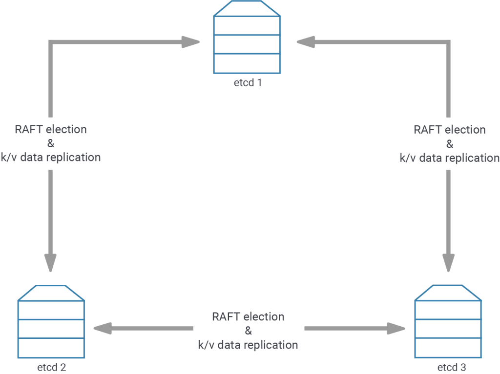
An example of one such tool is etcd, but there are others: consul, cockroach, with probably more to come. Several of them (etcd, consul) base their distributed decisions on the RAFT protocol, which includes a concept of leader election. As long as the members of the RAFT cluster can decide on a leader by voting, the DCS is able to function properly and accept changes to the data, as the leader of the current timeline is the one who decides if a request to change a variable can be accepted or not.
A good explanation and visual example of the RAFT protocol can be found here.

In etcd and consul, requests to change the keys and values can be formed to include conditions, like "only change this variable if it wasn't set to anything before" or "only change this variable if it was set to 42 before".

Patroni uses these requests to make sure that it only sets the leader-lock if it is not currently set, and it also uses it to extend the leader-lock, but only if the leader-lock matches its own member name. Patroni waits for the response by the DCS and then continues its work. For example, if Patroni fails to acquire the leader-lock, it will not promote or initialize the PostgreSQL instance.

On the other hand, should Patroni fail to renew the time to live that is associated with the leader-lock, it will stop the PostgreSQL database in order to demote it, because otherwise, it cannot guarantee that no other member of the cluster will attempt to become a leader after the leader key expired.

One of the steps  I described in the last blogpost - the step to deploy a Patroni cluster - sets up an etcd cluster:

However, that etcd cluster consists only of a single member.

Problems with single-member etcd clusters

In this scenario, as long as that single member is alive, it can elect itself to be the leader and thus can accept change requests. That's how our first Patroni cluster was able to function atop of this single etcd member.

But if this etcd instance were to crash, it would mean total loss of the DCS. Shortly after the etcd crash, the Patroni instance controlling the PostgreSQL primary would have to stop said primary, as it would be impossible to extend the time to live of the leader key.

To protect against such scenarios, wherein a single etcd failure or planned maintenance might disrupt our much desired highly-available PostgreSQL cluster, we need to introduce more members to the etcd cluster.

Three member etcd clusters

The number of cluster members that you choose to deploy is the most important consideration for deploying any DCS. There are two primary aspects to consider:

How likely is it that an etcd member fails or is offline for maintenance?

Usually, etcd members don't fail just by chance. So if you take care to avoid load spikes, and storage or memory issues, you'll want to consider at least two cluster members, so you can shut one down for maintenance.

How can a majority be found in the voting process?

By design, RAFT clusters require an absolute majority for a leader to be elected. This absolute majority depends upon the number of total etcd cluster members, not only those that are available to vote. This means that the number of votes required for a majority does not change when a member becomes unavailable. The number I just told you, two, was only a lower boundary for system stability and maintenance considerations.

In reality, a two member DCS will not work, because once you shut down one member, the other member will fail to get a majority vote for its leader candidacy, as 1 out of 2 is not more than 50%. If we want to be able to selectively shut members down for maintenance, we will have to introduce a third node, which can then partake in the leader election process. Then, there will always be two voters - out of the total three members - to choose a leader; two thirds is more than 50%, so the demands for absolute majority are met.

Placement of etcd cluster members in different data centers

The second most important consideration for etcd cluster deployments is the placement of the etcd nodes. Due to the aforementioned leader key expiry and the need for Patroni to refresh it at the beginning of each loop, and the fact that failure to achieve this will result in a forced stop of the leader, the placement of your etcd cluster members indirectly dictates how Patroni will react to network partitions and to the failure of the minority of nodes.

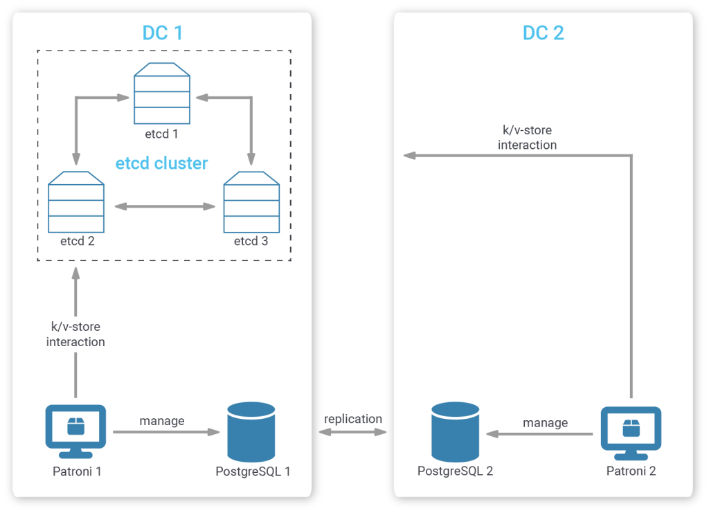
For starters, the simplest setup only resides in one data center (“completely biased cluster member placement”), so all Patroni and etcd members are not influenced by issues that cut off network access to the outside. At the same time, such a setup deals with the loss of the minority of etcd clusters in a simple way: it does not care - so long as there is still a majority of etcd members left that can talk to each other and to whom Patroni still can talk.

But if you'd prefer a cross-data center setup, where the replicating databases are located in different data centers, etcd member placement becomes critical.

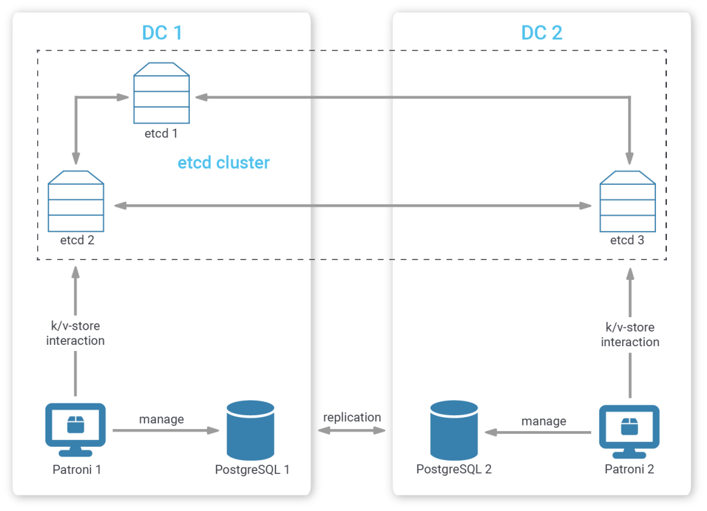
If you've followed along, you will agree that placing all etcd members in your primary data center (“completely biased cluster member placement”) is not wise. Should your primary data center be cut off from the outside world, there will be no etcd left for the Patroni members in the secondary data center to talk to, so even if they were in a healthy state, they could not promote. An alternative would be to place the majority of members in the first data center and a minority in the secondary one (“biased cluster member placement”).

Additionally, if one etcd member in your primary database is stopped - leaving your first data center without a majority of etcd members - and the secondary data center becomes unavailable as well, your database leader in the first data center will be stopped.

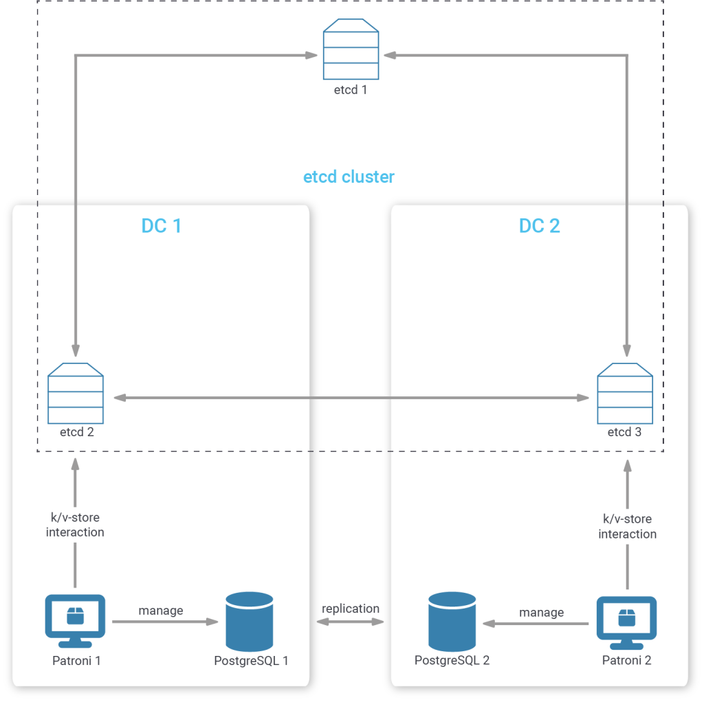
You could certainly manually mitigate this corner case by placing one etcd member in a tertiary position (“tertiary decider placement”), outside of both your first and second data center with a connection to each of them. The two data centers then should contain an equal number of etcd members.

This way, even if either data center becomes unavailable, the remaining data center, together with the tertiary etcd member can still come to a consensus.
Placing one etcd cluster member in a tertiary location can also have the added benefit that its perception of networking partitions might be closer to the way that your customers and applications perceive network partitions.

Placement of a tertiary cluster member as a decider

In the biased placement strategies mentioned above, consensus may be reached within a data center that is completely cut off from everything else. Placing one member in the tertiary position means that consensus can only be reached with the members in the data center that still have an intact uplink.

To increase the robustness of such a cluster even more, we can even place more than one node in a tertiary position, to mitigate against failures in a single tertiary member and network issues that could disconnect a single tertiary member.

You see, there are quite a lot of things to consider if you want to create a really robust etcd cluster. The above-mentioned examples are not an exhaustive list, and several other factors could influence your member placement needs. However, our experience has shown that etcd members seldom fail (unless there are disk latency spikes, or cpu-thrashing occurs) and that most customers want a biased solution anyway, as the primary data center is the preferred one. Usually, in biased setups, it is possible to add a new member to the secondary data center and exclude one of the members from the primary data center, in order  to move the bias to the second data center. In this way, you can keep running your database even if the first data center becomes completely inaccessible.

Setting up an etcd cluster

With the placement considerations out of the way, let’s look at how to create a simple etcd server. For demonstration purposes, we will constrain this setup to three hosts, 10.88.0.41, 10.88.0.42, 10.88.0.43.

There are a couple of different methods to configure and start (“bootstrap”) etcd clusters; I will outline two of them:

• The static bootstrap method requires knowledge of the network addresses of all cluster members. All addresses are then listed explicitly in the configuration file of each cluster member. This approach is great for learning and also easy to troubleshoot, as you can always look at the configuration file to see which hosts belong to the cluster.
• The discovery bootstrap method is a little more implicit and works better with setups where addresses may change regularly or where there may not even be real addresses available, for example: in container clusters where all containers can be reached using the same address, but via different ports.

Some settings need to be written into the etcd config regardless of the setup method.

Since etcd uses two different communication channels - one for peer communication with other etcd cluster members, another for client communication with users and applications - some of the configuration parameters may look almost identical, but they are nevertheless essential.

Each etcd member needs the following:

• name: A unique name within the etcd cluster.
• listen-peer-urls: A URL which states where etcd should listen for requests made by its peers. Usually, this is an IP or hostname reachable from the other etcd member’s hosts.
• listen-client-urls: A URL which states where etcd should listen for requests made by clients.  Usually, this is an IP or hostname reachable from the other etcd member’s hosts. If you also want to allow local connections by users and applications, you can add a URL based on the local IP address.
• initial-advertise-peer-urls: A URL which states which address other members of the cluster should use to connect to this etcd cluster member.
• advertise-client-urls: A URL which states which address clients should use if they want to connect to this etcd cluster member. Should only be an address reachable from the network, not a local one, even if this member listens to local connections.

The above parameters are required for each etcd member and they should be different for all etcd members, as they should all have different addresses -- or, at least, different ports.

Setting up an etcd cluster using static bootstrap

For the static bootstrap method, all etcd members additionally need the following parameters:

• initial-cluster-token: A token that is unique to your cluster. Simply generate some random characters.
• initial-cluster: By far the most important component required for a successful etcd bootstrap. This is a comma-separated string that lists all cluster members and their advertised peer-urls. Example: ‘centos_test_1=http://10.88.0.41:2380,centos_test_2=http://10.88.0.42:2380,centos_test_3=http://10.88.0.43:2380'

Now, if you start an instance of etcd on each of your nodes with fitting configuration files, they will try to talk to each other and - should your configuration be correct and no firewall rules are blocking traffic - bootstrap the etcd cluster.

As this blog post is already on the rather lengthy side, I have created an archive for you to download that contains logs that show the configuration files used as well as the output of the etcd processes.

Setting up an etcd cluster using discovery bootstrap

Another bootstrap approach, as I mentioned earlier, relies on an existing etcd cluster for discovery. Now, you don’t necessarily have to have a real etcd cluster. Keep in mind, that a single etcd process already acts as a cluster, albeit without high-availability. Alternatively, you can use the public discovery service located at discovery.etcd.io .

For the purpose of this guide, I will create a temporary local etcd cluster that can be reached by all members-to-be:

We don’t need any of the peer parameters here as this bootstrapper is not expected to have any peers.

A special directory and a key specifying the expected number of members of the new cluster both need to be created.
We will generate a unique discovery token for this new cluster:

The following call to curl creates the special size key, which implicitly creates the directory for cluster bootstrap in the bootstrapper’s key-value store:

The three etcd members-to-be now only need (besides the five basic parameters listed earlier) to know where to reach this discovery service, so the following line is added to all etcd cluster members-to-be:

Now, when the etcd instances are launched, they will register themselves into the directory that we created earlier. As soon as _config/size many members have gathered there, they will bootstrap a new cluster on their own.
At this point, you can safely terminate the bootstrapper etcd instance.

The output of the discovery bootstrap method along with the config files can also be found in the archive.

Checking etcd healthiness

To check whether the bootstrap was successful, you can call the etcdctl cluster-health command.

If you want to run this command somewhere other than on the hosts that contain the etcd members, you will have to specify the endpoints to which etcdctl should talk directly:

Running etcd as a Service

Usually, you'll want to run etcd as some sort of daemon that is started whenever your server is started, to protect against intermittent failures and negligence after planned maintenance.

If you've installed etcd via your operating system's package manager, a service file will already have been installed.
The service file is built in such a way that all of the necessary configuration parameters are loaded via environment variables. These can be set in the /etc/etcd/etcd.conf file and have a slightly different notation compared to the parameters that we've placed in YAML files in the examples above.
To convert the YAML configuration, you simply need to convert all parameter names to upper case and change dashes (-) to underscores (_) .

Caveats

If you try to follow this guide on Ubuntu or Debian and install etcd via apt, you will run into issues.
This is the result of the fact that everything that resembles a server automatically starts an instance through Systemd after installation has completed. You need to kill this instance, otherwise you won't be able to run your etcd cluster members on ports 2379 and 2380.

With the recent update to etcd 3.4, the v2 API of etcd is disabled by default. Since the etcd v3 API is however currently not useable with patroni (due to missing support for multiple etcd endpoints in the library, see this pull request), you'll need to manually re-enable support for the v2 API by adding enable-v2= true to your config file.

Conclusion

Bootstrapping an etcd server can be quite difficult if you run into it blindfolded. However, once the key concepts of etcd clusters are understood and you’ve learned what exactly needs to go into the configuration files, you can bootstrap an etcd cluster quickly and easily.

While there are lots of things to consider for member placement in more complex cross-data center setups, a simple three node cluster is probably fine for any testing environment and for setups which only span a single data center.

Do keep in mind that the cluster setups I demonstrated were stripped of any security considerations for ease of playing around. I highly recommend that you look into the different options for securing etcd. You should at least enable rolename and password authentication, and server certificates are probably a good idea to encrypt traffic if your network might be susceptible to eavesdropping attacks. For even more security, you can even add client certificates. Of course, Patroni works well with all three of these security mechanisms in any combination.

This post is part of a series.
Besides this post the following articles have already been published:
- PostgreSQL High-Availability and Patroni – an Introduction.
- Patroni: Setting up a highly availability PostgreSQL clusters

The series will also cover:
– configuration and troubleshooting
– failover, maintenance, and monitoring
– client connection handling and routing
– WAL archiving and database backups using pgBackrest
– PITR a patroni cluster using pgBackrest

By Kaarel Moppel

With the latest major version released, it's time to assess its performance. I've been doing this for years, so I have my scripts ready—it's more work for the machines. The v12 release introduces several enhancements, including a framework for changing storage engines, improved partitioning, smaller multi-column and repetitive value indexes, and concurrent re-indexing. These updates should boost performance for OLAP/Warehouse use cases, though OLTP improvements may be limited. Smaller indexes will help with large datasets. For detailed performance insights, check the summary table at the end or read further.

By the way - from a code change statistics point of view, the numbers look quite similar to the v11 release, with the exception that there is an increase of about 10% in the number of commits. This is a good sign for the overall health of the project, I think 🙂

Test queries

I decided to run 4 different test cases, each with a couple of different scale / client combinations. Scales were selected 100, 1000 and 5000 – with the intention that with 100, all data fits into shared buffers (which should provide the most accurate results), 1000 means everything fits into RAM (Linux buffer cache) for the used hardware and 5000 (4x RAM) to test if disk access was somehow improved. A tip - to quickly get the right “scaling factor” numbers for a target DB size, one could check out this post here.

The queries were all tied to or derived from the default schema generated by our old friend pgbench, and the 4 simulated test scenarios were as follows:

1) Default pgbench test mimicking an OLTP system (3x UPDATE, 1x SELECT, 1x INSERT)

 2) Default pgbench with a slightly modified schema - I decided to add a couple of extra indexes, since the release notes promised more effective storage of indexes with many duplicates and also for multi-column (compound) indexes, which surely has its cost. Extra index definitions were following:

 3) pgbench read-only (--select-only flag)

 4) Some home-brewed analytical / aggregate queries that I also used for testing the previously released PostgreSQL version, v11. The idea here is not to work with single records, but rather to scan over all tables / indexes or a subset on an index.

Test hardware / software

In order to get more reliable results this time, I used a dedicated old workstation machine that I have lying around as test hardware, instead of a cloud VM . . The machine is rather low-spec, but it at least has an SSD, so for comparing differences it should be totally fine. I actually did also try to use a cloud VM first (with a dedicated CPU), but the runtimes I got were so unpredictable on different runs of the same PG version that it was impossible to say anything conclusive.

CPU: 4x Intel(R) Core(TM) i5-6600 CPU @ 3.30GHz

RAM: 16GB

DISK: 256GB SSD

OS: Clean server install of Ubuntu 18.04 with some typical kernel parameter tuning for databases:

hdparm -W0 /dev/sda # disable write caching

vm.swappiness=1 # minimal swapping

vm.overcommit_memory=2 # no overcommit

vm.overcommit_ratio=99

For most tests, the disk parameters should not matter here either, as most used queries are quite read-heavy and data fits into shared buffers or RAM for most tests. This is actually what you want for an algorithmical comparison.

For running Postgres, I used the official Postgres project maintained [repo](https://wiki.postgresql.org/wiki/Apt) to install both 11.5 and 12.0. Concerning server settings (postgresql.conf), I left everything to defaults, except a couple of changes (see below) on both clusters, for reasons described in the comments.

Results

After running my test script for a couple of days (2h for each test case / scale / client count / PG version variation) on both clusters, here are the numbers for you to evaluate.

The scripts I used, doing all the hard work for me, can be found here by the way. For generating the percentage differences, you could use this query.

NB! Results were extracted directly from the tested PostgreSQL instances via the “pg_stat_statements” extension, so that the communication latency included in the pgbench results is not taken into account. Also note that the measured query “mean_times” are an average over various “client” parallelism counts:1-4 depending on the test. With analytical queries where “parallel query” kicks in-- with up to 2 extra workers per query-- it does not make sense to use more than $CPU_COUNT / 3 clients as some CPU starvation will otherwise occur (at default parallelism settings).

Testcase	Scale	v11 avg. “mean time” (ms)	v12 avg. “mean_time” (ms)	Mean time diff change	v11 “stddev”	v12 “stddev”	Stddev diff change
pgbench read-only	Buffers	0.0056	0.0058	3.6 %	0.002	0.002	0 %
	RAM	0.0605	0.0594	-2.2 %	0.4	0.4314	7.9 %
	Disk	0.3583	0.3572	-0.3 %	0.6699	0.6955	3.8 %
pgbench default UPDATE	Buffers	0.0196	0.0208	6.1 %	0.0063	0.0065	3.2 %
	RAM	0.1088	0.109	0.2 %	0.7573	0.8156	7.7 %
pgbench default INSERT	Buffers	0.034	0.0408	20 %	0.008	0.0222	177.5 %
	RAM	0.0354	0.0376	6.2	0.0109	0.0105	-3.7
pgbench extra indexes UPDATE	Buffers	0.0203	0.021	3.4	0.0067	0.0069	3
	RAM	0.1293	0.1283	-0.8	1.4285	1.1586	-18.9
pgbench extra indexes INSERT	Buffers	0.0447	0.0502	12.3	0.0111	0.0249	124.3
	RAM	0.0459	0.0469	2.2	0.0136	0.0152	11.8
Analytical Query 1	Buffers	551.81	556.07	0.8	39.76	33.22	-16.5
	RAM	2423.13	2374.30	-2	54.95	51.56	-2
Analytical Query 2	Buffers	996.08	984.09	-1.2	7.74	4.62	-40.2
	RAM	7521.1	7589.25	0.9	62.29	73.67	18.3
Analytical Query 3	Buffers	2452.23	2655.37	8.3	87.03	82.16	-5.6
	RAM	16568.9	16995.2	2.6	140.10	138.78	-0.9
Analytical Query 4	Buffers	876.72	906.13	3.4	41.41	37.49	-9.5
	RAM	4794.99	4763.72	-0.7	823.60	844.12	2.5
Total avg.				3.3			13.8

* pgbench default UPDATE means UPDATE on pgbench_accounts table here. pgbench_branches / tellers differences were discardable and the table would get too big.

Conclusion

As with all performance tests, skepticism is essential, as accurate measurement can be challenging. In our case, some SELECT queries averaged under 0.1 milliseconds, but larger standard deviations indicate randomness in tight timings. Additionally, the pgbench test is somewhat artificial, lacking real-world bloat and using narrow rows. I’d appreciate feedback if you've seen significantly different results or if my test setup seems reasonable. Interestingly, for the first time in years, average performance decreased slightly—by 3.3% for mean times and 13.8% for deviations. This could be expected since the storage architecture was revamped for future engine compatibility.

Also as expected, the new more space-saving index handling took the biggest toll on v12 pgbench INSERT performance (+10%)...but in the long run, of course, it will pay for itself nicely with better cache ratios / faster queries, especially if there are a lot of duplicate column values.

Another thing we can learn from the resulting query “mean times” (and this is probably even more important to remember than the 3% difference!) is that there are huge differences - roughly an order of magnitude - whether data fits into shared buffers vs memory, or memory vs disk. Thus the end with an obvious conclusion - for the best performance, investing in ample memory makes much more sense than a version upgrade!