Recently we had some clients who had the desire to store timeseries in PostgreSQL. One of the questions which interested them is related to calculating the difference between values in timeseries data. How can you calculate the difference between the current and the previous row?
To answer this question I have decided to share some simple queries outlining what can be done. Note that this is not a complete tutorial about analytics and windowing functions but just a short introduction to what can be done in general.
Let us load some sample data:
|
1 2 3 4 5 6 7 8 9 10 11 12 |
cypex=# CREATE TABLE t_oil ( region text, country text, year int, production int, consumption int ); cypex=# COPY t_oil FROM PROGRAM 'curl /secret/oil_ext.txt'; COPY 644 |
If you are a superuser you can use COPY ... FROM PROGRAM directly. Otherwise you have to load the text file in a different way.
If you want to calculate the difference between two rows, you can make use of the “lag” function. However, there is a question naturally arising here: If we want to access the previous row. What is the previous row? We will need some kind of order. To do that SQL provides the OVER-clause:
|
1 2 3 4 5 6 7 8 9 10 11 12 13 14 15 16 17 18 |
cypex=# SELECT country, year, production, lag(production, 1) OVER (ORDER BY year) FROM t_oil WHERE country = 'USA' LIMIT 10; country | year | production | lag ---------+------+------------+------- USA | 1965 | 9014 | USA | 1966 | 9579 | 9014 USA | 1967 | 10219 | 9579 USA | 1968 | 10600 | 10219 USA | 1969 | 10828 | 10600 USA | 1970 | 11297 | 10828 USA | 1971 | 11156 | 11297 USA | 1972 | 11185 | 11156 USA | 1973 | 10946 | 11185 USA | 1974 | 10461 | 10946 (10 rows) |
In my example I have ordered the data by year to make sure that the previous year can indeed be found in the previous row.
|
1 2 3 4 5 6 7 8 9 10 11 12 13 14 15 16 17 18 |
cypex=# SELECT country, year, production - lag(production, 1) OVER (ORDER BY year) AS diff FROM t_oil WHERE country = 'USA' LIMIT 10; country | year | diff ---------+------+------ USA | 1965 | USA | 1966 | 565 USA | 1967 | 640 USA | 1968 | 381 USA | 1969 | 228 USA | 1970 | 469 USA | 1971 | -141 USA | 1972 | 29 USA | 1973 | -239 USA | 1974 | -485 (10 rows) |
What is important to see here is that the first row contains a NULL entry because there is no known difference to the previous row.
What many people need is the difference between the current and the first row in the data set. PostgreSQL (or ANSI SQL in general to be more precise) offers the “first_value” function which returns the first row given the order provided by us. Here is how it works:
|
1 2 3 4 5 6 7 8 9 10 11 12 13 14 15 16 17 18 19 20 |
cypex=# SELECT t_oil.country, t_oil.year, t_oil.production, t_oil.production - first_value(t_oil.production) OVER (ORDER BY t_oil.year) AS diff_first FROM t_oil WHERE t_oil.country = 'USA'::text LIMIT 10; country | year | production | diff_first ---------+------+------------+------------ USA | 1965 | 9014 | 0 USA | 1966 | 9579 | 565 USA | 1967 | 10219 | 1205 USA | 1968 | 10600 | 1586 USA | 1969 | 10828 | 1814 USA | 1970 | 11297 | 2283 USA | 1971 | 11156 | 2142 USA | 1972 | 11185 | 2171 USA | 1973 | 10946 | 1932 USA | 1974 | 10461 | 1447 (10 rows) |
As you can see, in this case everything is relative to the first row.
The data looks correct so we can move on to the next examples.
But what happens if we start to look at two countries? If we order by year we might hit the wrong row. If we order by both columns we might still hit a row associated to a different country. The solution is the PARTITION BY clause. PostgreSQL will break up the data in various groups and calculate the difference again (for each group). Here is how it works:
|
1 2 3 4 5 6 7 8 9 10 11 12 13 14 15 16 17 18 |
cypex=# SELECT country, year, production, lag(production) OVER (PARTITION BY country ORDER BY year) AS diff FROM t_oil WHERE country IN ('Canada', 'Mexico') AND year < 1970; country | year | production | diff ---------+------+------------+------ Canada | 1965 | 920 | Canada | 1966 | 1012 | 920 Canada | 1967 | 1106 | 1012 Canada | 1968 | 1194 | 1106 Canada | 1969 | 1306 | 1194 Mexico | 1965 | 362 | Mexico | 1966 | 370 | 362 Mexico | 1967 | 411 | 370 Mexico | 1968 | 439 | 411 Mexico | 1969 | 461 | 439 (10 rows) |
In this example each group contains a NULL value because there is no “previous” value. This is proof that PostgreSQL handles the groups separately.
One more thing many people are interested in is the necessity to calculate moving averages. I decided to include this example in this post about differences because the problem pops up so often that it deserves some more attention. In many cases this type of operation is calculated on the application level which is clearly the wrong place to do because of performance reasons:
|
1 2 3 4 5 6 7 8 9 10 11 12 13 14 15 16 17 18 19 20 21 22 23 24 25 |
cypex=# SELECT country, year, production, avg(production) OVER (ORDER BY year ROWS BETWEEN 2 PRECEDING AND 2 FOLLOWING) AS mov FROM t_oil WHERE country IN ('Saudi Arabien') AND year BETWEEN 1975 AND 1990; country | year | production | mov ---------------+------+------------+----------------------- Saudi Arabien | 1975 | 7216 | 8465.6666666666666667 Saudi Arabien | 1976 | 8762 | 8487.7500000000000000 Saudi Arabien | 1977 | 9419 | 8758.4000000000000000 Saudi Arabien | 1978 | 8554 | 9369.2000000000000000 Saudi Arabien | 1979 | 9841 | 9668.0000000000000000 Saudi Arabien | 1980 | 10270 | 9176.4000000000000000 Saudi Arabien | 1981 | 10256 | 8455.8000000000000000 Saudi Arabien | 1982 | 6961 | 7394.4000000000000000 Saudi Arabien | 1983 | 4951 | 6060.6000000000000000 Saudi Arabien | 1984 | 4534 | 5051.0000000000000000 Saudi Arabien | 1985 | 3601 | 4578.6000000000000000 Saudi Arabien | 1986 | 5208 | 4732.4000000000000000 Saudi Arabien | 1987 | 4599 | 4952.6000000000000000 Saudi Arabien | 1988 | 5720 | 5653.4000000000000000 Saudi Arabien | 1989 | 5635 | 5764.7500000000000000 Saudi Arabien | 1990 | 7105 | 6153.3333333333333333 (16 rows) |
This defines the number of rows going into the aggregate function (in our case “avg”). The idea of a moving average is to flatten the curve and create a smoother line. The following picture shows how this works:
As you can see in the CYPEX visualization the moving average is a lot smoother than the rate underlying data. Saudi Arabia is a so called “swing producer”. Depending on the political situation the production rate might vary significantly so using a moving average actually makes a lot of sense.
However, there is more: Some of you might know that PostgreSQL supports composite data type. Basically every row can be seen as a single element containing various components. Usually a SELECT clause lists all desired fields, but you can also see a table as a single field as shown in the next example:
|
1 2 3 4 5 6 7 8 9 |
cypex=# SELECT t_oil, lag(t_oil) OVER (ORDER BY year) FROM t_oil WHERE country = 'Mexico' AND year IN (1980, 1981); t_oil | lag -----------------------------------------+----------------------------------------- ('North America',Mexico,1980,2129,1048) | ('North America',Mexico,1981,2553,1172) | ('North America',Mexico,1980,2129,1048) (2 rows) |
In this case all columns of a row are packed into a single field. You can use the “lag” function normally …
The trick now is: You can use “=” to compare two rows directly. Why is that important? Sometimes you want to see if two rows were imported twice or you simply want to know if two consecutive rows are identical. This is how it works:
|
1 2 3 4 5 6 7 8 9 |
cypex=# SELECT t_oil = lag(t_oil) OVER (ORDER BY year) FROM t_oil WHERE country = 'Mexico' AND year IN (1980, 1981); ?column? ---------- f (2 rows) |
It is possible to compare entire rows to each other. PostgreSQL will inspect one field after the other and only issue true in case all fields are the same. In other words: “lag” can even be abused to detect duplicate rows.
In order to receive regular updates on important changes in PostgreSQL, subscribe to our newsletter, or follow us on Facebook or LinkedIn.

(Updated 2023-02-24) There are three join strategies in PostgreSQL that work quite differently. If PostgreSQL chooses the wrong strategy, query performance can suffer a lot. This article explains the join strategies, how you can support them with indexes, what can go wrong with them and how you can tune your joins for better performance.
A join combines data from two relations. Such a relation can be a table (also called base relation) or the result of any plan node. For example, in a join like
|
1 2 3 4 |
SELECT ... FROM a JOIN (b LEFT JOIN c ON ...) ON ... |
the base relation a will be joined to the result of the join of b and c.
A relation can also be the result of an index scan. So when I say below that “PostgreSQL scans the relation sequentially”, I don't mean that there has to be a sequential scan on a table. It is just that PostgreSQL reads “the thing that is joined” in its entirety.
The execution plan for any join looks like this:
|
1 2 3 4 5 6 7 8 9 10 11 |
EXPLAIN (COSTS OFF) SELECT * FROM a JOIN b USING (id); QUERY PLAN ---------------------------- Hash Join Hash Cond: (a.id = b.id) -> Seq Scan on a -> Hash -> Seq Scan on b (5 rows) |
We call the upper of the joined relations (in this case the sequential scan on a) the outer relation of the join, and we call the lower relation (the hash computed from b) the inner relation.
A Cartesian product or cross join of two relations is what you get if you combine each row from one relation with each row of the other. The join condition is a filter that excludes some of these combinations. There are several ways to write a join condition, but all can be transformed to
|
1 |
a <join type> JOIN b ON <join condition> |
If the join condition is of the form
|
1 |
a.col1 <operator> b.col2 [AND ...] |
I call “a.col1” and “b.col2” join keys.
Note that for inner joins there is no distinction between the join condition and the WHERE condition, but that doesn't hold for outer joins.
This is the simplest and most general join strategy of all.
PostgreSQL scans the outer relation sequentially, and for each result row it scans the inner relation for matching rows.
Since we scan the outer relation sequentially, no index on the outer relation will help. But an index on the join key of the inner relation can speed up a nested loop join considerably.
Nested loop joins are particularly efficient if the outer relation is small, because then the inner loop won't be executed too often. It is the typical join strategy used in OLTP workloads with a normalized data model, where it is highly efficient. If the outer relation is large, nested loop joins are usually very inefficient, even if they are supported by an index on the inner relation.
Apart from that, it is the only join strategy that can be used if no join condition uses the = operator. So it also serves as a fall-back strategy if no other strategy can be used.
First, PostgreSQL scans the inner relation sequentially and builds a hash table, where the hash key consists of all join keys that use the = operator. Then it scans the outer relation sequentially and probes the hash for each row found to find matching join keys.
This is somewhat similar to a nested loop join. Building the hash table is an extra start-up effort, but probing the hash is much faster than scanning the inner relation.
Since we scan both relations sequentially, an index on the join condition will not help with a hash join.
Hash joins are best if none of the involved relations are small, but the hash table for the smaller table fits in work_mem. This is because otherwise PostgreSQL would build the hash in several batches and store them in temporary disk files, which hurts performance. In such cases the optimizer usually chooses a different join strategy like a merge join.
Looking up values in a hash table only works if the operator in the join condition is =, so you need at least one join condition with that operator.
In a merge join, PostgreSQL picks all join conditions with the = operator. It then sorts both tables by the join keys (which means that the data types must be sortable). Then it iterates through both sorted lists and finds matching entries.
An index on the sort keys can speed up sorting, so an index on the join keys on both relations can speed up a merge join. However, an explicit sort is often cheaper unless an index only scan can be used.
The optimizer usually chooses a merge join if the involved relations are both too big for a hash that fits into work_mem. So this is the best strategy for joining really large tables.
Like a hash join, a merge join is only feasible if there is at least one join condition with the = operator.
| Nested Loop Join | Hash Join | Merge Join | |
|---|---|---|---|
| Algorithm | For each outer relation row, scan the inner relation | Build a hash from the inner relation, scan the outer relation, probe the hash | Sort both relations and merge rows |
| Indexes that help | Index on the join keys of the inner relation | None | Indexes on the join keys of both relations |
| Good strategy if | the outer table is small | the hash table fits into work_mem |
both tables are large |
Choosing the wrong join strategy leads to bad performance:
In both cases, a bad row count estimate is the cause of the problem. So while the join may be where we spend most of the execution time, the cause is a misestimate that happened earlier on.
Find out what the best join strategy is (perhaps PostgreSQL is doing the right thing anyway). You can disable different join strategies temporarily with the SET command, which changes a parameter in your current database session:
|
1 2 3 |
SET enable_hashjoin = off; SET enable_mergejoin = off; SET enable_nestloop = off; |
Note that you cannot really disable nested loop joins, only discourage PostgreSQL from using them. If there is no join condition with an = operator, a nested loop join is the only way.
Tuning queries is often not a simple, straightforward task. However, here are some guidelines and ideas:
ANALYZE the table, perhaps with increased default_statistics_target, and see if that makes a difference. Try rewriting the query with simpler WHERE conditions to makes the optimizer's task easier.work_mem and see if you get a cheaper hash join.random_page_cost, effective_cache_size and effective_io_concurrency. That will allow it to price an index scan correctly.INCLUDE clause) and make sure that the table is vacuumed often enough.Understanding the 3 join strategies - nested loop join, hash join, and merge join - is crucial for anyone who wants to understand execution plans and tune queries. The art of query tuning cannot be conveyed in a single article, but I hope I could collect some relevant information here.
If you want to read more about tuning queries with joins, read some of our other articles on the topic, like Joining 1 million tables or Speeding up GROUP BY and joins.
Please leave your comments below. In order to receive regular updates on important changes in PostgreSQL, subscribe to our newsletter, or follow us on Twitter, Facebook, or LinkedIn.
After my last post about ltree and recursive data in PostgreSQL people have asked me privately about performance issues. To share this information, I decided to come up with a follow up post to discuss this topic in a bit more detail. WITH RECURSIVE in PostgreSQL is efficient. However, ltree does have its strengths as well. Let us take a closer look …
In preparation for a test I have created a table which contains a balanced tree:
|
1 2 3 4 5 6 7 8 9 10 11 12 13 14 15 16 |
test=# CREATE TABLE tree AS WITH RECURSIVE tree (id, parent, lvl) AS ( SELECT generate_series(1, 5) AS id, NULL :: int4 AS parent, 1 AS lvl UNION ALL SELECT n, id, lvl + 1 FROM tree, generate_series(power(5, lvl) :: int4 + (id - 1)*5 + 1, power(5, lvl) :: int4 + (id -1)*5 + 5 ) g(n) WHERE lvl < 10 ) SELECT * FROM tree ORDER BY id; |
There is a bit of magic involved here but let us not worry too much about the details at this point. Once the data is generated, you should see the following content in your table:
|
1 2 3 4 5 6 7 8 9 10 11 12 13 14 15 16 17 18 19 20 21 22 23 24 |
test=# SELECT * FROM tree LIMIT 20; id | parent | lvl ----+--------+----- 1 | | 1 2 | | 1 3 | | 1 4 | | 1 5 | | 1 6 | 1 | 2 7 | 1 | 2 8 | 1 | 2 9 | 1 | 2 10 | 1 | 2 11 | 2 | 2 12 | 2 | 2 13 | 2 | 2 14 | 2 | 2 15 | 2 | 2 16 | 3 | 2 17 | 3 | 2 18 | 3 | 2 19 | 3 | 2 20 | 3 | 2 (20 rows) |
|
1 2 3 4 5 |
test=# SELECT count(*) FROM tree; count ---------- 12207030 (1 row) |
12 million rows will be a nice way to show how efficient ltree can really be. As stated before, using a recursive query on this data might take a bit more time than running the query on prepared data. What you can do in the next listing is to resolve the tree and materialize an ltree column containing all the data. Make sure ltree is enabled in your database:
|
1 2 |
test=# CREATE EXTENSION ltree; CREATE EXTENSION |
Here is a materialized view containing the same data in a different format. The goal is to materialize the tree column to speed up searching:
|
1 2 3 4 5 6 7 8 9 10 11 12 13 14 15 16 |
test=# CREATE MATERIALIZED VIEW mat AS WITH RECURSIVE x AS ( SELECT id::text, parent::text, id::text::ltree AS mypath FROM tree WHERE parent IS NULL UNION ALL SELECT y.id::text, y.parent::text, ltree_addtext(x.mypath, y.id::text) AS mypath FROM x, tree AS y WHERE x.id::text = y.parent::text ) SELECT * FROM x; |
To access the materialized view efficiently, we have to create a Gist index on the ltree column:
|
1 2 |
test=# CREATE INDEX idx_mypath ON mat USING gist (mypath); CREATE INDEX |
Note that a btree is not what we are looking for here. A gist index is necessary. The reason is that a btree only supports sorting which is not quite what we need here in this case.
If your data is static materializing makes a lot of sense. In case your data changes frequently and in case you always need 100% correct results it is of course pretty counterproductive to pre-calculate data. However, let us take a look at the speed of the materialized case:
|
1 2 3 4 5 6 7 8 9 10 11 12 13 14 15 16 17 |
test=# explain analyze SELECT * FROM mat WHERE '4.21.129.770.4475.25499.143118.793712.4359182.23749035' @> mypath; QUERY PLAN ------------------------------------------------------------------------------------------------ Bitmap Heap Scan on mat (cost=161.88..4775.02 rows=1221 width=112) (actual time=0.117..0.117 rows=1 loops=1) Recheck Cond: ('4.21.129.770.4475.25499.143118.793712.4359182.23749035'::ltree @> mypath) Heap Blocks: exact=1 -> Bitmap Index Scan on idx_mypath (cost=0.00..161.57 rows=1221 width=0) (actual time=0.105..0.105 rows=1 loops=1) Index Cond: (mypath <@ '4.21.129.770.4475.25499.143118.793712.4359182.23749035'::ltree) Planning Time: 0.098 ms Execution Time: 0.270 ms (7 rows) |
The query executes in way less than a millisecond, which is exceptional.
Performance is king and we have written a lot about PostgreSQL performance in the past. One of the key aspects is VACUUM. Read on to find out how to enable and disable AUTOVACUUM.
In order to receive regular updates on important changes in PostgreSQL, subscribe to our newsletter, or follow us on Facebook or LinkedIn.
“If we had this data what would it mean?” - these kinds of questions can be answered using plain SQL. The technique you will need in PostgreSQL is a “hypothetical aggregate” which is of course part of the ANSI SQL standard. This post will show what an hypothetical aggregate is good for and how it works.
Just like min, max, sum, count, and so on a hypothetical aggregate is used in conjunction with a GROUP BY clause. The GROUP BY will split the data into small portions and the aggregation will be applied on each of those groups. To show how this works I have created 10 rows and split them into “even” and “off” numbers. The way to do it is “modulo 2”. Here is an example:
|
1 2 3 4 5 6 7 |
test=# SELECT x % 2 AS grp, array_agg(x) FROM generate_series(1, 10) AS x GROUP BY x % 2; grp | array_agg -----+-------------- 1 | {1,3,5,7,9} 0 | {2,4,6,8,10} (2 rows) |
As you can see PostgreSQL has stuffed all the data into two arrays. There is nothing fancy about it. We can use any other aggregate such as sum, avg, min, max, etc. However, I used array_agg to show you which values are taken into consideration to calculate the aggregate here.
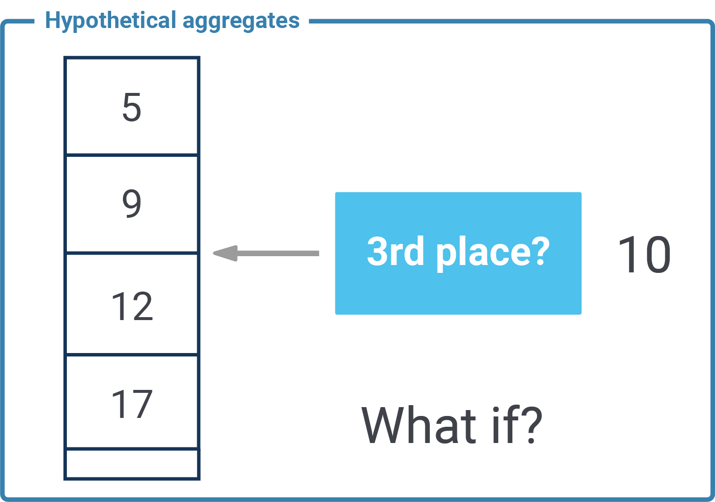
The main question now is: What is a hypothetical aggregate? Suppose we take the list of data in each group sort the values. Then we assume a hypothetical value (“as if it was there”) and see at which position it would end up. Here is an example:
|
1 2 3 4 5 6 7 8 9 |
test=# SELECT x % 2 AS grp, array_agg(x), rank(3.5) WITHIN GROUP (ORDER BY x) FROM generate_series(1, 10) AS x GROUP BY x % 2; grp | array_agg | rank -----+--------------+------ 0 | {10,2,4,6,8} | 2 1 | {9,7,3,1,5} | 3 (2 rows) |
If we take even numbers (2, 4, 6, 8, 10) in sorted 3.5 would be the 2nd entry. If we take odd numbers and sort them 3.5 would be the third value in the list. This is exactly what an hypothetical aggregate does.
Why would anybody want to use hypothetical aggregates in PostgreSQL? Here is an example: Suppose there is a sports event, and somebody is on the racing track. You want to know: If this racer reaches the finish line in 54 minutes, is he going to win? Finish as 10th? Or maybe last? A hypothetical aggregate will tell you that before the final score is inserted.
There are many more uses cases, but ranking is by far the most common and most widespread one.
If you want to know more about advanced SQL check out what we have to say about other fancy SQL stuff. Here is a post about speeding up aggregations by changing column orders.
Since SQL/MED (Management External Data) was implemented in PostgreSQL, hundreds of projects have emerged that try to connect PostgreSQL with other data sources. Just by doing a simple search on GitHub with the keys “postgres” + “fdw" you can figure that out.
Sadly not all extensions are well maintained and as a consequence they are deprecated. Fortunately, the extension that we have worked on db2_fdw and with which I've achieved to connect to DB2 is updated and works well for its main objective: Migrating db2's data to PostgreSQL.
From the next paragraph and if you follow our tips you'll also be able to read data from DB2 and expose it to PostgreSQL, so we'll see how to do it.
For this particular case, PostgreSQL 12.2 was used on Ubuntu 18.04.4 and the first important tip is that you need to install "IBM Data Server Client Packages". It must be configured properly before installing the extension. Here we got some tips.
|
1 2 3 4 5 |
# env |grep DB2 DB2_HOME=/home/user/sqllib DB2LIB=/home/user/sqllib/lib DB2INSTANCE=instance_name |
|
1 2 3 4 5 6 7 8 9 10 11 12 13 14 15 16 17 18 19 |
# db2 connect to testdb user db2inst1 using my_password Database Connection Information Database server = DB2/LINUXX8664 11.5.0.0 SQL authorization ID = DB2INST1 Local database alias = TESTDB # db2 => SELECT EMPLOYEE_ID, DATE_OF_BIRTH FROM EMPLOYEES LIMIT 5; EMPLOYEE_ID DATE_OF_BIRTH ----------- ------------- 1. 08/19/1971 2. 06/15/1978 3. 12/23/1979 4. 11/14/1979 5. 02/08/1977 5 record(s) selected. |
And remember that if DB2 instance is in another network you should also add it to pg_hba.conf.
Same steps as when installing other extensions from the source code.
|
1 2 3 |
# git clone https://github.com/wolfgangbrandl/db2_fdw.git # make # sudo make install |
Now we'll create the extension in PostgreSQL, verify it and that's it.
|
1 2 3 4 5 6 7 8 9 10 |
pgdb=# create extension db2_fdw; pgdb=# dx List of installed extensions Name | Version | Schema | Description ---------+---------+------------+------------------------------------- db2_fdw | 1.0 | public | foreign data wrapper for DB2 access plpgsql | 1.0 | pg_catalog | PL/pgSQL procedural language (2 rows) |
If the previous warm-up was successful then there is nothing stopping us now. So to wrap db2 inside PostgreSQL follow the following steps:
|
1 |
pgdb=# CREATE SERVER testdb FOREIGN DATA WRAPPER db2_fdw OPTIONS (dbserver 'testdb'); |
|
1 |
pgdb=# CREATE USER MAPPING FOR PUBLIC SERVER testdb OPTIONS (user 'db2inst1', password 'my_password'); |
Important: db2inst1 and my_password are DB2 database server username and password, respectively. In the next item we will see that the name of the schema is: DB2INST1. They are values created by default by the db2 wizard setup. In your particular case these values may differ.
|
1 |
pgdb=# IMPORT FOREIGN SCHEMA 'DB2INST1' FROM SERVER testdb INTO public; |
|
1 2 3 4 5 6 7 8 9 |
pgdb=# SELECT EMPLOYEE_ID, DATE_OF_BIRTH FROM EMPLOYEES LIMIT 5; employee_id | date_of_birth -------------+--------------- 1 | 1971-08-19 2 | 1978-06-15 3 | 1979-12-23 4 | 1979-11-14 5 | 1977-02-08 (5 rows) |
As you can see we've achieved to connect to the DB2 instance and get data, now we'll see what these kinds of tables look like in PostgreSQL:
|
1 2 3 4 5 6 7 8 9 10 11 12 13 |
pgdb=# d public.employees Foreign table 'public.employees' Column | Type | Collation | Nullable | Default | FDW options ---------------+-------------------------+-----------+----------+---------+-------------- employee_id | numeric | | not null | | (key 'true') first_name | character varying(1000) | | not null | | (key 'true') last_name | character varying(1000) | | not null | | (key 'true') date_of_birth | date | | not null | | (key 'true') phone_number | character varying(1000) | | not null | | (key 'true') junk | character(254) | | not null | | (key 'true') t | text | | | | Server: testdb FDW options: (schema 'DB2INST1', 'table' 'EMPLOYEES') |
Pay special attention to FDW options, which tell us that this table is not from here, but we can work with it.
In fact, we can perform CRUD operations on these tables, and we can even have detailed information about the query through explain. It makes a call to db2expln and gives us information about the cost and access that is used internally in the DB2 engine. We can see that below.
|
1 2 3 4 5 6 7 8 9 |
pgdb=# EXPLAIN SELECT EMPLOYEE_ID, DATE_OF_BIRTH FROM EMPLOYEES LIMIT 5; QUERY PLAN --------------------------------------------------------------------------------------------------- Limit (cost=10000.00..10050.00 rows=5 width=36) -> Foreign Scan on employees (cost=10000.00..20000.00 rows=1000 width=36) DB2 query: SELECT /*30a9058135496929abaa9e871e651ec4*/ r1.'EMPLOYEE_ID', r1.'DATE_OF_BIRTH' FROM 'DB2INST1'.'EMPLOYEES' r1 DB2 plan: Estimated Cost = 70.485092 DB2 plan: Estimated Cardinality = 1000.000000 (5rows) |
In conclusion, we can say that db2_fdw is a mature, simple and reliable extension to migrate data from DB2 to PostgreSQL as you have seen here. If you found it interesting that how fdw is useful to connect to external data then I invite you to look at this post.
Read on to find out more in Hans-Jürgen Schönig's blog Understanding Lateral Joins in PostgreSQL.
In order to receive regular updates on important changes in PostgreSQL, subscribe to our newsletter, or follow us on Facebook or LinkedIn.
This blog is about table functions and performance. PostgreSQL is a really powerful database and offers many features to make SQL even more powerful. One of these impressive things is the concept of a composite data type. In PostgreSQL a column can be a fairly complex thing. This is especially important if you want to work with server side stored procedures or functions. However, there are some details people are usually not aware of when making use of stored procedures and composite types.
Before we dive into the main topic of this post, I want to give you a mini introduction to composite types in general:
|
1 2 3 4 5 6 7 8 9 10 11 |
test=# CREATE TYPE person AS (id int, name text, income numeric); CREATE TYPE I have created a simple data type to store persons. The beauty is that the composite type can be seen as one column: test=# SELECT '(10, 'hans', 500)'::person; person ------------------ (10,' hans',500) (1 row) |
However, it is also possible to break it up again and represent it as a set of fields.
|
1 2 3 4 5 |
test=# SELECT ('(10, 'hans', 500)'::person).*; id | name | income ----+------+-------- 10 | hans | 500 (1 row) |
|
1 2 3 4 5 6 7 8 |
test=# CREATE TABLE data (p person, gender char(1)); CREATE TABLE test=# d data Table 'public.data' Column | Type | Collation | Nullable | Default --------+--------------+-----------+----------+--------- p | person | | | gender | character(1) | | | |
As you can see the column type is “person”.
Armed with this kind of information we can focus our attention on performance. In PostgreSQL a composite type is often used in conjunction with stored procedures to abstract values passed to a function or to handle return values.
Why is that important? Let me create a type containing 3 million entries:
|
1 2 3 4 5 6 7 |
test=# CREATE TABLE x (id int); CREATE TABLE test=# INSERT INTO x SELECT * FROM generate_series(1, 3000000); INSERT 0 3000000 test=# vacuum ANALYZE ; VACUUM |
pgstattuple is an extension which is especially useful if you want to detect bloat in a table. It makes use of a composite data type to return data. Installing the extension is easy:
|
1 2 |
test=# CREATE EXTENSION pgstattuple; CREATE EXTENSION |
What we want to do next is to inspect the content of “x” and see the data (all fields). Here is what you can do:
|
1 2 3 4 5 6 7 |
test=# explain analyze SELECT (pgstattuple('x')).*; QUERY PLAN ------------------------------------------------------------------------------------------- Result (cost=0.00..0.03 rows=1 width=72) (actual time=1909.217..1909.219 rows=1 loops=1) Planning Time: 0.016 ms Execution Time: 1909.279 ms (3 rows) |
Wow, it took close to 2 seconds to generate the result. Why is that the case? Let us take a look at a second example:
|
1 2 3 4 5 6 7 8 |
test=# explain analyze SELECT * FROM pgstattuple('x'); QUERY PLAN ---------------------------------------------------------------------------------------------- Function Scan on pgstattuple (cost=0.00..0.01 rows=1 width=72) (actual time=212.056..212.057 rows=1 loops=1) Planning Time: 0.019 ms Execution Time: 212.093 ms (3 rows) |
Ooops? What happened? If we put the query in the FROM-clause the database is significantly faster. The same is true if we use a subselect:
|
1 2 3 4 5 6 7 |
test=# explain analyze SELECT (y).* FROM (SELECT pgstattuple('x') ) AS y; QUERY PLAN ----------------------------------------------------------------------------------------- Result (cost=0.00..0.01 rows=1 width=32) (actual time=209.666..209.666 rows=1 loops=1) Planning Time: 0.034 ms Execution Time: 209.698 ms (3 rows) |
Let us analyze the reasons for this behavior!
The problem is that PostgreSQL expands the FROM-clause. It actually turns (pgstattuple('x')) into …
|
1 2 3 4 5 6 |
… (pgstattuple('x')).table_len, (pgstattuple('x')).tuple_count, (pgstattuple('x')).tuple_len, (pgstattuple('x')).tuple_percent, … |
As you can see, the function is called more often in this case which of course explains the runtime difference. Therefore it makes a lot of sense to understand what is going on under the hood here. The performance improvement can be quite dramatic. We have seen a couple of cases in PostgreSQL support recently which could be related to this kind of behavior.
If you want to know more about performance consider checking out my blog post about CREATE INDEX and parallelism.
In order to receive regular updates on important changes in PostgreSQL, subscribe to our newsletter, or follow us on Facebook or LinkedIn.
A while ago, I wrote about B-tree improvements in v12. PostgreSQL v13, which will come out later this year, will feature index entry deduplication as an even more impressive improvement. So I thought it was time for a follow-up.
If the indexed keys for different table rows are identical, a GIN index will store that as a single index entry. The pointers to the several table rows (tuple IDs) are stored in the posting list of that entry.
In contrast, B-tree indexes used to store an index entry for each referenced table row. This makes maintenance faster but can lead to duplicate index entries. Now commit 0d861bbb70 has changed that by introducing deduplication of index entries for B-tree indexes.
The big difference is that duplicate index entries can still occur in B-tree indexes. GIN indexes have to integrate new entries into the posting list every time, which makes data modifications less efficient (this is mitigated by the pending list). In contrast, PostgreSQL deduplicates B-tree entries only when it would otherwise have to split the index page. So it has to do the extra work only occasionally, and only when it would have to do extra work anyway. This extra work is balanced by the reduced need for page splits and the resulting smaller index size.
Oh yes, it does. Every UPDATE creates a new version of a table row, and each row version has to be indexed. Consequently, even a unique index can contain the same index entry multiple times. The new feature is useful for unique indexes because it reduces the index bloat that normally occurs if the same table row is updated frequently.
Deduplication results in a smaller index size for indexes with repeating entries. This saves disk space and, even more importantly, RAM when the index is cached in shared buffers. Scanning the index becomes faster, and index bloat is reduced.
If you want to make use of the new feature after upgrading with pg_upgrade, you'll have to REINDEX promising indexes that contain many duplicate entries. Upgrading with pg_dumpall and restore or using logical replication rebuilds the index, and deduplication is automatically enabled.
If you want to retain the old behavior, you can disable deduplication by setting deduplicate_items = off on the index.
I'll use the same test case as in my previous article:
|
1 2 3 4 5 6 7 8 9 10 11 12 13 14 15 16 |
CREATE TABLE rel ( aid bigint NOT NULL, bid bigint NOT NULL ); ALTER TABLE rel ADD CONSTRAINT rel_pkey PRIMARY KEY (aid, bid); CREATE INDEX rel_bid_idx ON rel (bid); INSERT INTO rel (aid, bid) SELECT i, i / 10000 FROM generate_series(1, 20000000) AS i; /* set hint bits and calculate statistics */ VACUUM (ANALYZE) rel; |
The interesting index here is rel_bid_idx. I'll measure its size, then the size after a REINDEX. Finally, I'll execute the following query several times:
|
1 2 3 |
DO $$BEGIN PERFORM * FROM rel WHERE bid < 100::bigint; END;$$; |
This executes an index scan without actually transferring the result to the client. I'll measure the time with psql's timing on the client side.
I'll run that test on PostgreSQL v12 and v13. As a comparison, I'll do the same thing with a GIN index on bid (this requires the btree_gin contrib module).
| v13 B-tree index | v12 B-tree index | v12 GIN index | |
|---|---|---|---|
| size | 126MB | 408MB | 51MB |
size after REINDEX |
133MB | 429MB | 47MB |
| query duration | 130ms | 130ms | 140ms |
In my example, the deduplicated B-tree index is more than three times smaller than the v12 index, although it is still considerably larger than the GIN index.
The performance is comparable. I observed a bigger variance in the execution time with the deduplicated index, which I cannot explain.
This feature is another nice step ahead for PostgreSQL's B-tree indexes!
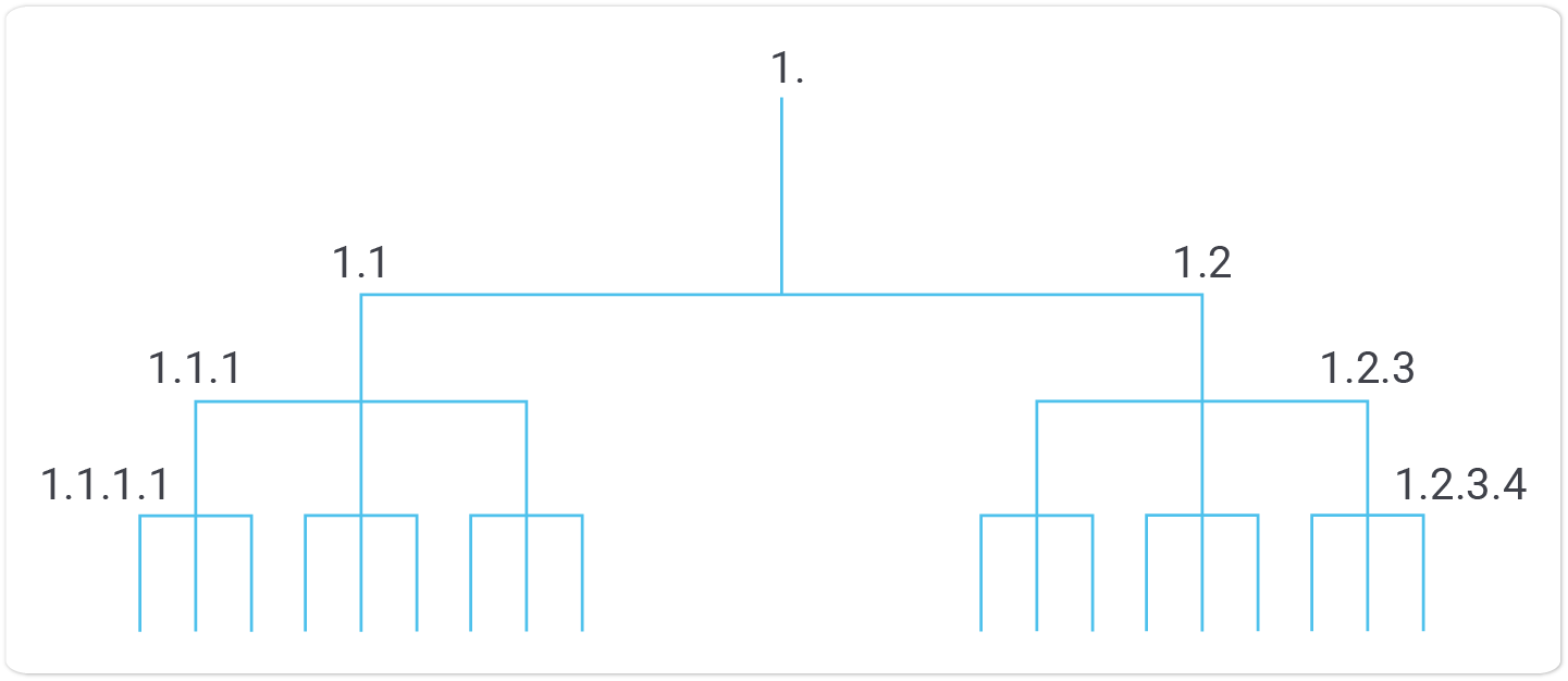
A hierarchical query is an SQL query that handles hierarchical model data such as the structure of organizations, living species, and a lot more. All important database engines including PostgreSQL, Oracle, DB2 and MS SQL offer support for this type of query.
However, in some cases hierarchical queries can come with a price tag. This is especially true if trees are deep, complex and therefore require some effort by the database engine to handle all this data. Simple queries are usually not a problem but if trees grow out of proportion “WITH RECURSIVE” (ANSI SQL) and “CONNECT BY” (the old Oracle implementation) might start to be an issue.
The ltree module is part of the standard PostgreSQL contrib package which can be found on most servers and can therefore be loaded as a normal extension. It should also be provided by most cloud services including Amazon RDS, AWS and Microsoft Azure.
Ltree implements a data type ltree for representing labels of data stored in a hierarchical tree-like structure. This blog will show how this module can be used to speed up some quite common use cases.
The first thing you have to do is to make sure that the ltree extension is loaded into your database server. CREATE EXTENSION will do the job. Then I have created a simple hierarchical structure that has a parent and a child value. This is the standard approach to store this kind of data:
|
1 2 3 4 5 6 7 8 |
CREATE EXTENSION ltree; CREATE TABLE t_orga ( parent_code text, child_code text, UNIQUE (parent_code, child_code) ); |
In the next step I have created some test data.
(more on that a little later):
|
1 2 3 4 5 6 7 8 9 10 11 12 13 14 15 |
INSERT INTO t_orga VALUES (NULL, 'A'), ('A', 'B'), ('B', 'C'), ('B', 'D'), ('D', 'E'), ('C', 'F'), ('C', 'G'), ('E', 'H'), ('F', 'I'), ('I', 'J'), ('G', 'K'), ('K', 'L'), ('L', 'M') ; |
|
1 2 3 4 5 6 7 8 9 10 11 12 13 14 15 16 17 |
test=# SELECT * FROM t_orga ; parent_code | child_code -------------+------------ | A A | B B | C B | D D | E C | F C | G E | H F | I I | J G | K K | L L | M (13 rows) |
In my data “A” is on top of the food chain (this is why the parent label is NULL in this case). Basically this data structure is already enough to figure out if you want to know all employees working in “A → B → C”. The question is: If your organization or your data in general is pretty constant - can we do better? Plants, animals and so on are not shifted around between classes on a regular basis. Elephants won't be plants tomorrow and a rose will not turn into an animal either. These data sets are quite stable and we can therefore apply to trick to query them faster.
Before taking a look at the trickery I have promised I want to focus your attention on some simple ltree examples so that you can understand how ltree works in general:
|
1 2 3 4 5 |
test=# SELECT 'A.B.C'::ltree; ltree ------- A.B.C (1 row) |
|
1 2 3 4 5 |
test=# SELECT ltree_addtext('A.B.C'::ltree, 'D'); ltree_addtext --------------- A.B.C.D (1 row) |
|
1 2 3 4 5 |
test=# SELECT ltree_addtext(NULL::ltree, 'D'); ltree_addtext --------------- (1 row) |
|
1 2 3 4 5 |
test=# SELECT ltree_addtext(''::ltree, 'D'); ltree_addtext --------------- D (1 row) |
As you can see, ltree is a “.”-separated kind of list. You can append values easily. But you have to be careful: You can append to the list if it contains an empty string. If the value is NULL you cannot append. The same is true for other stuff in PostgreSQL as well, and you should be aware of this issue. What is also important is that ltree can hold labels - not arbitrary strings. Here is an example:
|
1 2 |
test=# SELECT ltree_addtext('A'::ltree, '.'); ERROR: syntax error at position 0 |
Armed with this information we can create a materialized view which pre-aggregates some data.
In PostgreSQL you can pre-aggregate data using a materialized view. In this case we want to pre-calculate the hierarchy of data and store it as a separate column:
|
1 2 3 4 5 6 7 8 9 10 11 |
CREATE MATERIALIZED VIEW t_orga_mat AS WITH RECURSIVE x AS ( SELECT *, child_code::ltree AS mypath FROM t_orga WHERE parent_code IS NULL UNION ALL SELECT y.parent_code, y.child_code, ltree_addtext(x.mypath, y.child_code) AS mypath FROM x, t_orga AS y WHERE x.child_code = y.parent_code ) SELECT * FROM x; |
To do that I have used WITH RECURSIVE which is the standard way of doing this kind of operation. How does it work? The SELECT inside the recursion has two components. Something before the UNION ALL and something after it. The first part selects the starting point of the recursion. We basically want to start at the beginning. In our case parent_code has to be NULL - this tells us that we are on top of the food chain. All the data is selected, and a column is added at the end. The first line will only contain the child_code as it is the first entry on top of the tree.
The second part will take the result created by the first part and join it. Then the last column is extended by the current value. We do that until the join does not yield anything anymore.
Yes, it can. Basically one has to use UNION instead of UNION ALL to prevent a nested loop from happening. However, in case of ltree this does not work because to do that, the data type must support hashing which ltree does not. In other words: You must be 100% sure that the dataset does NOT contain loops.
The materialized view will create this kind of result:
|
1 2 3 4 5 6 7 8 9 10 11 12 13 14 15 16 17 |
test=# SELECT * FROM t_orga_mat; parent_code | child_code | mypath -------------+------------+--------------- | A | A A | B | A.B B | C | A.B.C B | D | A.B.D D | E | A.B.D.E C | F | A.B.C.F C | G | A.B.C.G E | H | A.B.D.E.H F | I | A.B.C.F.I G | K | A.B.C.G.K I | J | A.B.C.F.I.J K | L | A.B.C.G.K.L L | M | A.B.C.G.K.L.M (13 rows) |
As you can see the last column has all the higher levels. The main question now is: How can we query this data? Here is an example:
|
1 2 3 4 5 6 7 8 |
test=# SELECT * FROM t_orga_mat WHERE 'A.B.C.G' @> mypath; parent_code | child_code | mypath -------------+------------+--------------- C | G | A.B.C.G G | K | A.B.C.G.K K | L | A.B.C.G.K.L L | M | A.B.C.G.K.L.M (4 rows) |
We are looking for everybody in “A → B → C → G”. Of course ltree provides many more operators which can be found in the official documentation.
Keep in mind that the table is small so PostgreSQL would naturally use a sequential scan and not consider the index for efficiency reasons. It only does so when the table is larger. To encourage the optimizer to choose an index, we can make sequential scans super expensive:
|
1 2 3 4 5 6 7 8 |
test=# SET enable_seqscan TO off; SET test=# explain SELECT * FROM t_orga_mat WHERE 'A.B.C.G' @> mypath; QUERY PLAN --------------------------------------------------------------------------- Index Scan using idx_mat on t_orga_mat (cost=0.13..8.15 rows=1 width=96) Index Cond: (mypath <@ 'A.B.C.G'::ltree) (2 rows) |
You can see that PostgreSQL is using the desired index to speed up this kind of data.
Hierarchical data is important. We have covered this topic in the past already. If you want to find out more, read our post about WITH RECURSIVE and company organization.