Adjusting maintenance_work_mem

After testing shared_buffers recently, I decided to do a little more testing on our new office desktop PC (8 core AMD CPU, 4 GHZ, 8 GB RAM and a nice 128 GB Samsung 840 SSD). All tests were conducted on the SSD drive.

This time I tested the impact of maintenance_work_mem on indexing speed. To get started I created half a billion rows using the following simple code snippet:

BEGIN;

DROP SEQUENCE IF EXISTS seq_a;
CREATE SEQUENCE seq_a CACHE 10000000;


CREATE TABLE t_test (
     id         int4    DEFAULT nextval('seq_a'),
     name       text
);

INSERT INTO t_test (name) VALUES ('hans');

DO
$$
   DECLARE
      i      int4;

   BEGIN
      i := 0;
      WHILE i < 29
      LOOP
        i := i + 1;
        INSERT INTO t_test (name) SELECT name FROM t_test;
      END LOOP;
   END;
$$ LANGUAGE 'plpgsql';

SELECT count(*) FROM t_test;

COMMIT;

 

VACUUM t_test;

Once the data is loaded we can check the database size. The goal of the data set is to clearly exceed the size of RAM so that we can observe more realistic results.

In our case we got 24 GB of data:

test=# SELECT pg_size_pretty(pg_database_size('test'));
 pg_size_pretty
----------------
 24 GB
(1 row)

The number of rows is: 536870912

sorted input:

The point is that our data set has an important property: We have indexed the integer column. This implies that the input is already sorted.

Each index is built like that:

DROP INDEX idx_id;
CHECKPOINT;
SET maintenance_work_mem TO '32 MB';

CREATE INDEX idx_id ON t_test (id);

We only measure the time of indexing. A checkpoint is requested before we start building the index to make sure that stuff is forced to disk before, and no unexpected I/O load can happen while indexing.

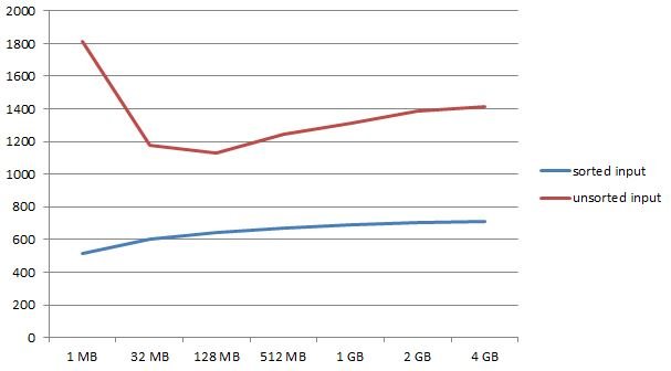
The results are as follows:

1 MB: 516 sec

32 MB: 605 sec

128 MB: 641 sec

512 MB: 671 sec

1 GB: 688 sec

2 GB: 704 sec

4 GB: 709 sec

The interesting part here is that we can see the top performing index creating with very little memory. This is not totally expected but it makes sense given the way things work. We see a steady decline, given more memory.

unsorted input:

Let us repeat the test using unsorted data now.

We create ourselves a new table containing completely random order of the same data:

test=# CREATE TABLE t_random AS SELECT * FROM t_test ORDER BY random();
SELECT 536870912

Let us run those index creations again:

1 MB: 1810 sec

32 MB: 1176 sec

128 MB: 1130 sec

512 MB: 1244 sec

1 GB: 1315 sec

2 GB: 1385 sec

4 GB: 1411 sec

As somewhat expected, the time needed to create indexes has risen. But: In this case we cannot see the best performer on the lower or the upper edge of the spectrum but somewhere in the middle at 128 MB of RAM. Once the system gets more memory than that, we see a decline, which is actually quite significant, again.

From my point of view this is a clear statement that being too generous is clearly not the best strategy.

Of course, results will be different on different hardware and things depend on the nature of data as well as on the type of index (Gist and GIN would behave differently) in use. However, for btrees the picture seems clear.