A lot has been written about effective_cache_size in postgresql.conf and about PostgreSQL performance in general. However, few people know what this famous parameter really does. Let me share some more insights.
The idea behind SQL is actually quite simple: The end user sends a query and the optimizer is supposed to find the best strategy to execute this query. The output of the optimizer is what people call an “execution plan”. The question now is: What makes one execution plan better than some other plan? What is it that makes a strategy greater than some other strategy? In PostgreSQL everything boils down to the concept of “costs”. The planner will assign costs to every operation. At the end of the day the cheapest plan is selected and executed.
The magic is therefore in the way the optimizer handles costs. That is exactly what effective_cache_size is all about.
To achieve good performance it is important to figure out whether to use an index or not. A question often asked is: Why not always use an index? Traversing and index might not be cheap at and using an index does not mean that there is no need to touch the table as well. The optimizer therefore has to decide whether to go for an index or not.
The way costs are estimated depend on various factors: Amount of I/O needed, number of operators called, number of tuples processed, selectivity, and a lot more. However, what is the cost of I/O? Obviously it makes a difference if data is already in cache or if data has to be read from disk. That brings us to the idea behind effective_cache_size which tells the optimizer how much cache to expect in the system. The important part is that “cache” is not only the amount of memory knows about (this part is pretty clear). The system also has to consider the size of the filesystem cache, CPU caches, and so on. effective_cache_size is the sum of all those caching components. What you will learn in this post is how the optimizer uses this kind of information.
Before we lose ourselves in theoretical explanation it makes sense to dig into a practical example. For the purpose of this blog I have generated two tables:
|
1 2 3 4 5 6 7 8 9 10 11 12 |
test=# CREATE TABLE t_random AS SELECT id, random() AS r FROM generate_series(1, 1000000) AS id ORDER BY random(); SELECT 1000000 test=# CREATE TABLE t_ordered AS SELECT id, random() AS r FROM generate_series(1, 1000000) AS id; SELECT 1000000 test=# CREATE INDEX idx_random ON t_random (id); CREATE INDEX test=# CREATE INDEX idx_ordered ON t_ordered (id); CREATE INDEX test=# VACUUM ANALYZE ; VACUUM |
Mind that both tables contain the same set of data. One table is ordered - the other one is not. Let us set the effective_cache_size to a really small value. The optimizer will assume that there is really not much memory in the system:
|
1 2 3 4 5 6 7 8 9 10 |
test=# SET effective_cache_size TO '1 MB'; SET test=# SET enable_bitmapscan TO off; SET test=# explain SELECT * FROM t_random WHERE id < 1000; QUERY PLAN --------------------------------------------------------------------------------- Index Scan using idx_random on t_random (cost=0.42..3611.96 rows=909 width=12) Index Cond: (id < 1000) (2 rows) |
Normally PostgreSQL would go for a bitmap index scan, but we want to see what happens in case of an index scan. Therefore we turn bitmap scans off (= making them insanely expensive to the optimizer).
Let us compare the plan with the one we have just seen before:
|
1 2 3 4 5 6 7 8 |
test=# SET effective_cache_size TO '1000 GB'; SET test=# explain SELECT * FROM t_random WHERE id < 1000; QUERY PLAN -------------------------------------------------------------------------------- Index Scan using idx_random on t_random (cost=0.42..3383.99 rows=909 width=12) Index Cond: (id < 1000) (2 rows) |
As you can see, the price of the index scan has gone down. Why is that relevant? We have to see costs as “relative”. The absolute number is not important - it is important how expensive a plan is compared to some other plan. If the price of a sequential scan stays the same and the price of an index scan goes down relative to a seq scan PostgreSQL will favor indexing more often than it otherwise would. This is exactly what effective_cache_size at its core is all about: Making index scans more likely if there is a lot of RAM around.
When people talk about postgresql.conf and effective_cache_size they are often not aware of the fact that the parameter does not always work miracles. The following scenario shows when there is no impact:
|
1 2 3 4 5 6 7 8 9 10 11 12 13 14 15 16 17 |
test=# SET effective_cache_size TO '1 MB'; SET test=# explain SELECT * FROM t_ordered WHERE id < 1000; QUERY PLAN ---------------------------------------------------------------------------------- Index Scan using idx_ordered on t_ordered (cost=0.42..39.17 rows=1014 width=12) Index Cond: (id < 1000) (2 rows) test=# SET effective_cache_size TO '1000 GB'; SET test=# explain SELECT * FROM t_ordered WHERE id < 1000; QUERY PLAN ---------------------------------------------------------------------------------- Index Scan using idx_ordered on t_ordered (cost=0.42..39.17 rows=1014 width=12) Index Cond: (id < 1000) (2 rows) |
The table statistics used by the optimizer contain information about physical “correlation”. If correlation is 1 (= all data is sorted perfectly on disk) effective_cache_size will NOT change anything.
The same is true if the is only one column as shown in the next example:
|
1 2 3 4 5 6 7 8 9 10 11 12 13 14 15 16 17 18 19 |
test=# ALTER TABLE t_random DROP COLUMN r; ALTER TABLE test=# SET effective_cache_size TO '1 MB'; SET test=# explain SELECT * FROM t_ordered WHERE id < 1000; QUERY PLAN ---------------------------------------------------------------------------------- Index Scan using idx_ordered on t_ordered (cost=0.42..39.17 rows=1014 width=12) Index Cond: (id < 1000) (2 rows) test=# SET effective_cache_size TO '1000 GB'; SET test=# explain SELECT * FROM t_ordered WHERE id < 1000; QUERY PLAN ---------------------------------------------------------------------------------- Index Scan using idx_ordered on t_ordered (cost=0.42..39.17 rows=1014 width=12) Index Cond: (id < 1000) (2 rows) |
That comes as a surprise to most users and therefore I considered it worth mentioning.
I found it useful to use a simple formula to get a rough estimate for a good setting:
effective_cache_size = RAM * 0.7
Some people have also used 0.8 successfully. Of course this is only true when we are talking about a dedicated database server. Feel free to experiment.
In order to receive regular updates on important changes in PostgreSQL, subscribe to our newsletter, or follow us on Facebook or LinkedIn.
By Kaarel Moppel
Recently I was asked if there’s a rule of thumb / best practice for setting the fillfactor in Postgres - and the only answer I could give was to decrease it “a bit” if you do lots and lots of updates on some table. Good advice? Well, it could be better - this kind of coarse quantization leaves a lot of room for interpretation and possible adverse effects. So to have a nicer answer ready for the next time, I thought it would be nice to get some real approximate numbers. Time to conjure up some kind of a test! If you already know what fillfactor does, then feel free to skip to the bottom sections. There you'll find some numbers and a rough recommendation principle.
But first a bit of theory for the newcomers - so what does fillfactor do and how do you configure it? Simon says:
The fillfactor for a table is a percentage between 10 and 100. 100 (complete packing) is the default. When you specify a smaller fillfactor, INSERT operations pack table pages only to the indicated percentage. The remaining space on each page is reserved for updating rows on that page. This gives UPDATE a chance to place the updated copy of a row on the same page as the original, which is more efficient than placing it on a different page. For a table whose entries are never updated, complete packing is the best choice. However, in heavily updated tables smaller fillfactors are appropriate. This parameter cannot be set for TOAST tables.
In short, it’s a per table (or index!) parameter that directs Postgres to initially leave some extra disk space on data pages unused. Later UPDATE-s could use it, touching ultimately only one data block, thus speeding up such operations. And besides normal updates it also potentially (depending on if updated columns are indexed or not) enables another special, and even more beneficial, type of update, known as HOT updates. The acronym means Heap Only Tuples, i.e. indexes are not touched.
There's quite a simple base concept: how densely should we initially “pack” the rows? (Many other database systems also offer something similar.) Not much more to it - but how to set it? Sadly (or probably luckily) there’s no global parameter for that and we need to change it “per table”. Via some SQL, like this:
|
1 2 |
-- leave 10% of block space unused when inserting data ALTER TABLE pgbench_accounts SET (fillfactor = 90); |
As the documentation mentions, for heavily updated tables we can gain on transaction performance by reducing the fillfactor (FF). But in what range should we adjust it and how much? Documentation doesn’t take a risk with any numbers here. Based on my personal experience, after slight FF reductions small transaction improvements can usually be observed. Not immediately, but over some longer period of time (days, weeks). And as I haven’t witnessed any cases where it severely harms performance, you can certaily try such FF experiments for busy tables. But in order to get some ballpark numbers, I guess the only way is to set up a test...
As per usual, I modified some test scripts I had lying around, that use the default pgbench schema and transactions, which should embody a typical simple OLTP transaction with lots of UPDATE-s...so exactly what we want. The most important parameter (relative to hardware, especially memory) for pgbench transaction performance is the “scale factor”, so here I chose different values covering 3 cases - initial active data set fits almost into RAM, half fits and only a fraction (ca 10%) fits. Tested fillfactor ranges were 70, 80, 90, 100.
Test host: 4 CPU i5-6600, 16GB RAM, SATA SSD
PostgreSQL: v12.2, all defaults except: shared_buffers set to 25% of RAM, i.e. 4GB, checkpoint_completion_target = 0.9, track_io_timing = on, wal_compression = on, shared_preload_libraries=’pg_stat_statements’
Pgbench: scales 1000/2500/10000, 12h runtime for each scale / FF combination, 2 concurrent sessions.
Query latencies were measured directly in the database using the pg_stat_statement extension, so they should be accurate.
By the way, if you wonder why I’m not using the latest Postgres version v12.3 for my testing (which is normally the way to go) - all these combinations took a week to run through and although a new release appeared during that time I thought it’s not worth it as I didn’t see anything relevant from the release notes.
Performance has many aspects and even for a bit of a simplistic pgbench test we could measure many things - maybe most important for us in this fillfactor context are the frequent updates on our biggest table that we want to optimize. But let’s not also forget about the effect of our fillfactor changes on the Postgres background processes, worse caching rates etc, so for completeness let’s also look at the total Transactions per Seconds numbers. Remember - 1 pgbench default transaction includes 3 updates (2 mini-tables + 1 main), 1 insert into the write-only history table + 1 select from the main table by PK.
So here the effects on pgbench_accounts UPDATE mean time as measured via pg_stat_statements in milliseconds with global TPS in parentheses:
| Data scale | FF=100 | FF=90 | FF=80 | FF=70 |
| Mem. | 5.01 (374) | 4.80 (389) | 4.89 (382) | 4.98 (376) |
| 2x Mem. | 5.31 (363) | 5.33 (359) | 5.38 (357) | 5.42 (353) |
| 10x Mem. | 6.45 (249) | 5.67 (282) | 5.61 (284) | 5.72 (279) |
What can we learn from the test data? Although it seems that there was some slight randomness in the tests (as 2x Mem test actually made things minimally slower), on the whole it seems that decreasing FF a bit also improves performance “a bit”! My general hunch has something to it, even 🙂 On average a 10% boost, when decreasing FF by 10 or 20%. It's not game changing, but it could make a visible difference.
And the second learning - don’t overdo it! As we see that FF 70% clearly deteriorates the update performance instead of improving it, with all scaling factors.
My try at a rule of thumb - when your active / hot data set is a lot bigger than the amount of RAM, going with fillfactor 90% seems to be a good idea. Don’t forget - there are still no free lunches out there. When optimizing for fast updates on table X, we pay some of the winnings back with global TPS numbers. Our tables will be somewhat bigger, we lose a bit on cache hit ratios, and also background workers like the autovacuum daemon have more scanning to do. So for smaller data vs RAM ratios, the benefits are not particularly visible. You might even lose slightly in global TPS numbers.
Some more thoughts - I’m pretty sure that if I had tuned autovacuum to be more aggressive, we would have seen some more performance improvement. In spite of decreasing the FF, the pgbench_accounts table was still growing considerably during the testing (~35% at biggest scale) even at FF 70%. And the same for old spinning disks - the potential for additional winnings with fillfactor tuning is even bigger there compared to SSD-s, because fillfactor helps to reduce exactly the Achilles heel of rotating disks - the costly random access.
Read more about performance improvements:
LIKE and ILIKE are two fundamental SQL features. People use those things all over the place in their application and therefore it makes sense to approach the topic from a performance point of view. What can PostgreSQL do to speed up those operations and what can be done in general to first understand the problem and secondly to achieve better PostgreSQL database performance.
In this blog post you will learn mostly about Gist and GIN indexing. Both index type can handle LIKE as well as ILIKE. These index types are not equally efficient, so it makes sense to dig into the subject matter and figure out what is best when.
Before we get started I have created some sample data. To avoid searching the web for sample data I decided to generate some data. A simple md5 hash is more than sufficient to prove my point here.
|
1 2 3 4 5 6 |
test=# CREATE TABLE t_hash AS SELECT id, md5(id::text) FROM generate_series(1, 50000000) AS id; SELECT 50000000 test=# VACUUM ANALYZE; VACUUM |
Let us take a look at the data. What we got here are 50 million ids and their hashes. The following listing shows what the data looks like in general:
|
1 2 3 4 5 6 7 8 9 10 11 12 13 14 |
test=# SELECT * FROM t_hash LIMIT 10; id | md5 ----+---------------------------------- 1 | c4ca4238a0b923820dcc509a6f75849b 2 | c81e728d9d4c2f636f067f89cc14862c 3 | eccbc87e4b5ce2fe28308fd9f2a7baf3 4 | a87ff679a2f3e71d9181a67b7542122c 5 | e4da3b7fbbce2345d7772b0674a318d5 6 | 1679091c5a880faf6fb5e6087eb1b2dc 7 | 8f14e45fceea167a5a36dedd4bea2543 8 | c9f0f895fb98ab9159f51fd0297e236d 9 | 45c48cce2e2d7fbdea1afc51c7c6ad26 10 | d3d9446802a44259755d38e6d163e820 (10 rows) |
Let us turn our attention to LIKE: The Following query selects a substring which exists in the data only once. Mind that the percent symbol is not just at the end but also at the beginning of the pattern:
|
1 2 3 4 5 6 7 8 |
test=# timing Timing is on. test=# SELECT * FROM t_hash WHERE md5 LIKE '%e2345679a%'; id | md5 ----------+---------------------------------- 37211731 | dadb4b54e2345679a8861ab52e4128ea (1 row) Time: 4767.415 ms (00:04.767) |
On my iMac, the query takes 4.7 seconds to complete. In 90+% of all applications out there this is already way too long. The user experience is already going to suffer and there is a good chance that a long running query like that will already increase the load on your server quite substantially.
To see what is going on under the hood I decided to include the execution plan of the SQL statement:
|
1 2 3 4 5 6 7 8 9 |
test=# explain SELECT * FROM t_hash WHERE md5 LIKE '%e2345679a%'; QUERY PLAN ------------------------------------------------------------------------------ Gather (cost=1000.00..678583.88 rows=5000 width=37) Workers Planned: 2 -> Parallel Seq Scan on t_hash (cost=0.00..677083.88 rows=2083 width=37) Filter: (md5 ~~ '%e2345679a%'::text) (4 rows) Time: 11.531 ms |
Because of the size of the table the PostgreSQL query optimizer will go for a parallel query. That is basically a good thing because the execution time is cut in half. But: It also means that we are readily sacrificing two CPU cores to answer this query returning just a single row.
The reason for bad performance is that the table is actually quite large, and the database has to read it from the beginning to the end to process the request:
|
1 2 3 4 5 6 |
test=# dt+ List of relations Schema | Name | Type | Owner | Size | Description --------+--------+-------+-------+---------+------------- public | t_hash | table | hs | 3256 MB | (1 row) |
Reading 3.2 GB to fetch just a single is now to efficient at all.
So what can we do to solve this problem?
Fortunately PostgreSQL offers a module which can do a lot of trickery in the area of pattern matching. The pg_trgm extension implements “trigrams” which is a way to help with fuzzy search. The extension is part of the PostgreSQL contrib package and should therefore be present on the vast majority of systems:
|
1 2 3 |
test=# CREATE EXTENSION pg_trgm; CREATE EXTENSION Time: 77.216 ms |
As you can see enabling the extension is easy. The natural question arising now is: What is a trigram? Let us take a look and see:
|
1 2 3 4 5 |
test=# SELECT show_trgm('dadb4b54e2345679a8861ab52e4128ea'); show_trgm --------------------------------------------------------------------------------------------------------------------------------------------- {' d',' da',128,1ab,234,28e,2e4,345,412,456,4b5,4e2,52e,54e,567,61a,679,79a,861,886,8ea,9a8,a88,ab5,adb,b4b,b52,b54,dad,db4,e23,e41,'ea '} (1 row) |
What you can observe is that a trigram is like a sliding 3 character window. All these tokens will show up in the index as you will see later on.
To index LIKE the pg_trgm module supports two PostgreSQL index types: Gist and GIN. Both options will be evaluated.
What many people do to speed up fuzzy searching in PostgreSQL is to use Gist indexes. Here is how this type of index can be deployed:
|
1 2 3 |
test=# CREATE INDEX idx_gist ON t_hash USING gist (md5 gist_trgm_ops); CREATE INDEX Time: 2383678.930 ms (39:43.679) |
What you can already see is that the index needs quite some time to build. What is important to mention is that even higher maintenance_work_mem settings will NOT speed up the process. Even with 4 GB of maintenance_work_mem the process will take 40 minutes.
What is also noteworthy is that the index is really large:
|
1 2 3 4 5 6 |
test=# di+ List of relations Schema | Name | Type | Owner | Table | Size | Description --------+----------+-------+-------+--------+---------+------------- public | idx_gist | index | hs | t_hash | 8782 MB | (1 row) |
Keep in mind the table is just 3.5 GB - the index is 2.5 times larges.
But, indexes will always make things faster, right? Well, actually no...
|
1 2 3 4 5 6 |
test=# SELECT * FROM t_hash WHERE md5 LIKE '%e2345679a%'; id | md5 ----------+---------------------------------- 37211731 | dadb4b54e2345679a8861ab52e4128ea (1 row) Time: 105506.064 ms (01:45.506) |
We have really “optimized” the query? Instead of 4.7 seconds PostgreSQL needs almost 2 minutes to do the job. Why is that the case? Let us take a look what the execution plan has to say:
|
1 2 3 4 5 6 7 8 9 |
test=# explain SELECT * FROM t_hash WHERE md5 LIKE '%e2345679a%'; QUERY PLAN ---------------------------------------------------------------------------- Bitmap Heap Scan on t_hash (cost=495.30..18812.90 rows=5000 width=37) Recheck Cond: (md5 ~~ '%e2345679a%'::text) -> Bitmap Index Scan on idx_gist (cost=0.00..494.05 rows=5000 width=0) Index Cond: (md5 ~~ '%e2345679a%'::text) (4 rows) Time: 13.433 ms |
The PostgreSQL optimizer has decided to go for a “Bitmap Index Scan”. So maybe a direct index scan is better?
|
1 2 3 4 5 6 7 8 9 10 11 12 13 |
test=# SET enable_bitmapscan TO off; SET Time: 11.302 ms test=# explain analyze SELECT * FROM t_hash WHERE md5 LIKE '%e2345679a%'; QUERY PLAN ----------------------------------------------------------------------------- Index Scan using idx_gist on t_hash (cost=0.55..20428.04 rows=5000 width=37) (actual time=13750.850..99070.510 rows=1 loops=1) Index Cond: (md5 ~~ '%e2345679a%'::text) Planning Time: 0.074 ms Execution Time: 99070.618 ms (4 rows) Time: 99072.657 ms (01:39.073) |
Actually the query is still going to show horrible execution times.
In short: A Gist index might not be the right thing to use here. It takes ages to create, it is large, it is a lot slower than a sequential scan.
Fortunately the pg_trgm extensions offers a second operator class to get the job done. GIN indexes are usually used to for PostgreSQL Full Text search (FTS). Let us see if we can win in case of LIKE and ILIKE as well? Before we do that we reset the current connection and drop the old index:
|
1 2 3 4 5 6 |
test=# DISCARD ALL; DISCARD ALL Time: 12.000 ms test=# DROP INDEX idx_gist; DROP INDEX Time: 3123.336 ms (00:03.123) |
In the next step a new index is created:
|
1 2 3 |
test=# CREATE INDEX idx_gin ON t_hash USING gin (md5 gin_trgm_ops); CREATE INDEX Time: 698063.038 ms (11:38.063) |
On my machine it takes 11 minutes which is a lot but actually a lot faster than the " rel="noopener" target="_blank">Gist index creation. However, index creation only happens once so we should not worry too much in this case. What is usually more important (usually) is query execution time:
|
1 2 3 4 5 6 7 8 9 10 11 12 13 14 15 |
test=# explain analyze SELECT * FROM t_hash WHERE md5 LIKE '%e2345679a%'; QUERY PLAN ------------------------------------------------------------------------------ Bitmap Heap Scan on t_hash (cost=2270.75..20588.36 rows=5000 width=37) (actual time=74.592..74.593 rows=1 loops=1) Recheck Cond: (md5 ~~ '%e2345679a%'::text) Heap Blocks: exact=1 -> Bitmap Index Scan on idx_gin (cost=0.00..2269.50 rows=5000 width=0) (actual time=74.584..74.584 rows=1 loops=1) Index Cond: (md5 ~~ '%e2345679a%'::text) Planning Time: 0.066 ms Execution Time: 74.665 ms (7 rows) Time: 75.031 ms |
Wow, we can run the query in 75 milliseconds instead of 4.7 seconds respectively 1 minute and 45 seconds. This is a major leap forward. A small index for man - a giant leap for database performance.
As expected the query returns exactly one row:
|
1 2 3 4 5 6 7 |
test=# SELECT * FROM t_hash WHERE md5 LIKE '%e2345679a%'; id | md5 ----------+---------------------------------- 37211731 | dadb4b54e2345679a8861ab52e4128ea (1 row) Time: 74.487 ms |
What you have seen so far is that the GIN index has solved the problem. However, you might still need a second index here. GIN does not speed up the “=” operator. So if you are looking for a normal lookup you will need a second index as shown in the next example:
|
1 2 3 4 5 6 7 8 9 10 |
test=# CREATE INDEX idx_btree ON t_hash (md5); CREATE INDEX Time: 274778.776 ms (04:34.779) test=# di+ List of relations Schema | Name | Type | Owner | Table | Size | Description --------+-----------+-------+-------+--------+---------+------------- public | idx_btree | index | hs | t_hash | 2816 MB | public | idx_gist | index | hs | t_hash | 2807 MB | (2 rows) |
A btree is needed to speed up normal comparisons. A GIN index alone will not be sufficient for that:
|
1 2 3 4 5 6 7 |
test=# SELECT * FROM t_hash WHERE md5 = 'dadb4b54e2345679a8861ab52e4128ea'; id | md5 ----------+---------------------------------- 37211731 | dadb4b54e2345679a8861ab52e4128ea (1 row) Time: 0.379 ms |
PostgreSQL offers truly powerful indexing strategies. There is a lot more to discover than just btree indexes. Gist and GIN have their strengths too. GIN is especially useful for all kinds of full text operations while Gist is ideal for geometric data (GIS).
If you want to find out more about GIN indexes check out my posting about the GIN posting list and VACUUM behavior. It will be very useful if you are looking for good GIN performance.
After exactly half a year (seems to be a pattern already) since the last major release of pgwatch2 Open Source PostgreSQL monitoring tool, I'm glad to announce that another set of useful features and improvements have found their way into the pgwatch2 code repository!
The new version is incremented to v1.8.0 and content-wise, it's mostly about new features and improvements with some bugfixes thrown in - but previous versions have proven to be very stable. So here is a short list of the most significant changes since the last major release, v1.7. Note that not all changes are covered here so please go to the GitHub changelog if details are of interest to you, i.e. if you are upgrading from an existing installation.
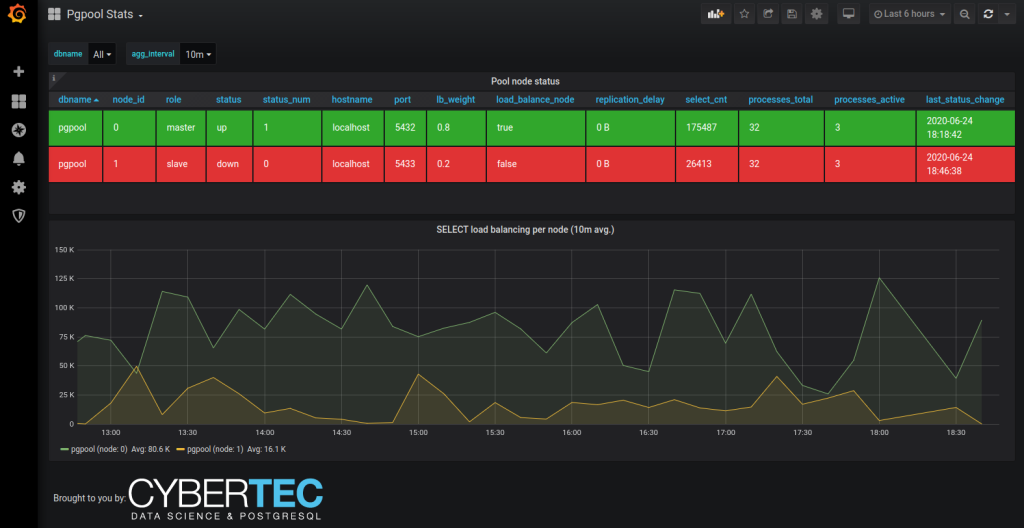
The main feature for me this time would be Pgpool support. Although I usually try to avoid using it if possible but lots of our customers still do, so that over time there have been quite some requests on that and finally it's here. From the technical side it makes use of the "SHOW POOL_NODES" and "SHOW POOL_PROCESSES" commands (being extensible via SQL still as all metrics) and glues the data together so that it's especially useful to monitor load balancing setups where Pgpool has a tendency to promptly detach nodes from load balancing even when some milder errors are encountered.
Besides the regular and obvious PostgreSQL v13 support (touching up some metrics, most notably the pg_stat_statements related ones) the second most notable feature is the addition of another option to store metrics in a PostgreSQL database (5 different storage schemas now for Postgres + InfluxDB + Prometheus + Graphite), specifically targeted support for the very popular TimescaleDB extension. Usage of this extension was, of course, already possible previously as it does not fiddle too much with the SQL access layer, but the users had to roll up the sleeves and take care of details such as registering hypertables, chunking and retention – now this is all automatic! After the initial rollout of the schema of course.
...that although it will most probably work, I do not recommend using TimescaleDB for pgwatch2 before version v1.5 as then the "killer feature" of built-in compression for historic chunks was added – before that there are no gains to be expected against standard Postgres given some pgwatch2 auto-partitioned storage schema was used. Talking about gains - according to my testing the compression really helps a lot for bigger monitoring setups and savings of 5-10x in storage space can be achieved! The query times did not really change though as the latest data that the dashboards are showing is not yet compressed and still mostly cached.
This new feature allows pausing of certain metrics collection on certain days/times, with optional time zone support if monitoring stuff across the pond for example. The main use case is that on some servers we might have very performance critical timespans and we don't want to take any chances – as indeed some bloat monitoring metrics (not enabled by default though) can cause considerable disk load.
Such metrics collection pausing can be both defined on the "metric" level, i.e. applies for all hosts using that metric during the specified interval, or on "metric-host" level so that it's really targeted. A sample declaration for one such "pausing" interval can be seen here.
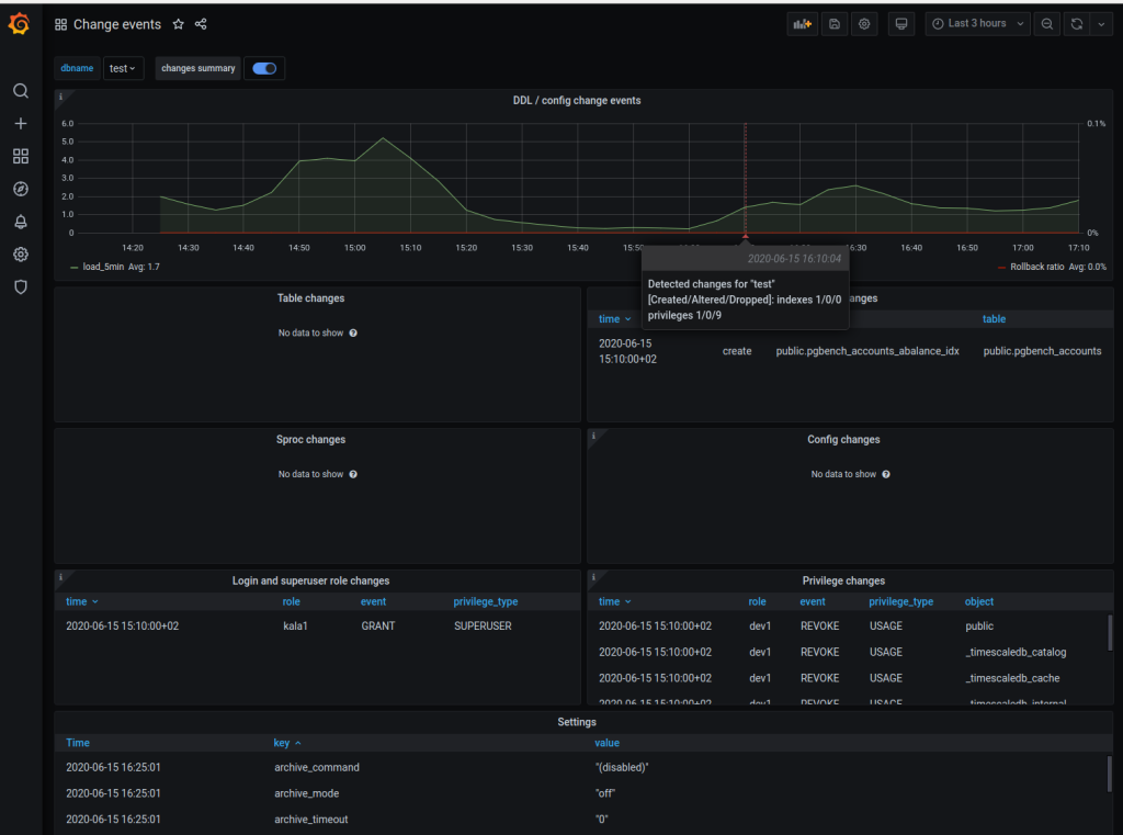
Previously already table, index, function and server configuration changes were tracked (if the "change_detection" metric was enabled) but now we also monitor object access privileges on tables / views, schemas, functions, databases and the roles system - login roles, granted role associations and most importantly Superusers. The new information is made available on a new panel on the already existing "Change events" dashboard.
This gatherer improvement aims to reduce query load in case we're monitoring many or all databases of a single instance. Previously all metrics were always fetched directly from the DB...but in reality a lot of them are global / instance level metrics (WAL, replication, CPU load, etc) and we could re-use the information. And exactly this is now happening for the 'continuous' DB types out of the box. Caching period is by default 30s, but customizable via the –instance-level-cache-max-seconds param or PW2_INSTANCE_LEVEL_CACHE_MAX_SECONDS env. variable.
So far all the configuration operations in the optional Web UI component were only possible "per monitored db" - so it was a lot tedious clicking to disable / enable all hosts temporarily or to start using some other pre-set configs. So now there bulk change buttons for enabling, disabling, password and preset config change over all defined databases.
We were already able to define metrics SQL-s based on PostgreSQL version and primary / replica state but now there's another dimension – versions of specific extensions. The use cases should be rare of course and the whole change was actually a bit unplanned and needed only because one extension we use for index recommendations changed its API so much that we needed this new dimension for a workaround in cases when both old and new versions of the extensions were used on separate DB hosts. But anyways I'm pretty sure we're going to see such breaking extension API changes also in the future so better be already prepared for the real life.
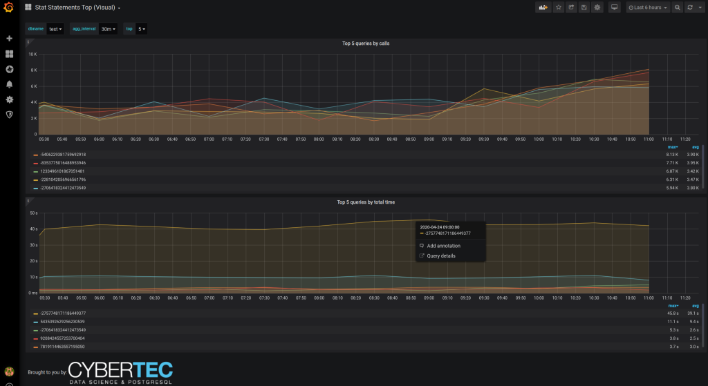
There was already a tabular dashboard for the data extracted via the pg_stat_statements but now the new 'Stat Statements Top (Visual)' shows the top resource consuming queries in graph format so it's visually easier to grasp and also shows changes over time. There are also links to the 'Single query details' dash making use of the new Grafana "data links" feature. NB! Defined only for Postgres data sources.
Another one based on pg_stat_statements data (the most useful performance troubleshooting extension certainly deserves that) – the new 'Stat statements Top (Fast)' differentiates from the standard 'Stats Statements Top' by "assuming" that the during the selected time range the internal statistics were not reset on the monitored DB nor was there a server crash. In this case we don't need to use the somewhat costly window functions but simple aggregates and this is a real perceptible win when looking at weekly or larger time spans. NB! Defined only for Postgres data sources.
The existing table_stats / table_io_stats metrics relying on pg_stat(io)_user_tables system views, were changed so that for natively partitioned tables (PG 10+) the purely virtual parent also gets one stats row, summarizing all child stats. For me this is a huge usability improvement actually for monitoring heavily partitioned tables and I wonder why Postgres doesn't do the same out of the box and leaves it to the user to write some relatively ugly recursive queries like the one here.
The "reco" engine now has 3 new checks / suggestion – against possibly forgotten disabled table triggers, against too frequent checkpoint requests (this is logged into the server log also by the way as warning) and against inefficient full indexing (seen quite often) on columns where most values are NULL actually and one could possibly benefit a lot from partial indexes, leaving out those NULL-s.
As AWS is here to stay would make sense to “play nice” with their Postgres services I guess – so now there’s a two new preset configs for that purpose. They’re unimaginatively called ‘aurora’ and ‘rds’ and leave out some metrics that AWS for some reason has decided not to expose or implement in case of Aurora.
This in short enables storing of slightly different metric definitions under one metric name. The only case for this currently is the new ‘stat_statements_no_query_text’ metric that is a more secure variation of the normal ‘stat_statements’ metric without the query texts, but not to define separate dashboards etc, the data is stored under the same name. To make use of this feature define a metric level attribute called ‘metric_storage_name’ and the metric will be routed correctly on storage.
These two tools are quite popular in the community so now there are according metrics and PL/Python metric fetching helpers to execute the “info” commands on the OS level and give back the results via SQL so that it could be dashboarded / alerted on in Grafana as for all other metrics.
As we see more and more Logical Replication usage for various application architecture goals adding a built-in metric makes a lot of sense. It’s called 'logical_subscriptions' and is included now in the 'full' preset config.
Now after RPM / DEB install and Python dependency installations (not included, needs pip install -r requirements.txt) one can immediately launch also the Web UI. There’s also a SystemD template to auto-start on boot.
And as always, please do let us know on GitHub if you’re still missing something in the tool or are experiencing difficulties - any feedback would be highly appreciated to make the product better for everyone!
Project GitHub link – here
Full changelog – here.
DEMO site here.
pgwatch2 is constantly being improved and new features are added. Learn more >>
¡Hola, queridos amigos! We've released several valuable features for pg_timetable in May. It's summer already, and time is flying fast! I hope all of you are well and safe, as well as your families and friends.
Here I want to introduce what's new and how that is useful briefly. If you are unfamiliar with pg_timetable, the best PostgreSQL scheduler in the world, you may read previous posts about it. ?
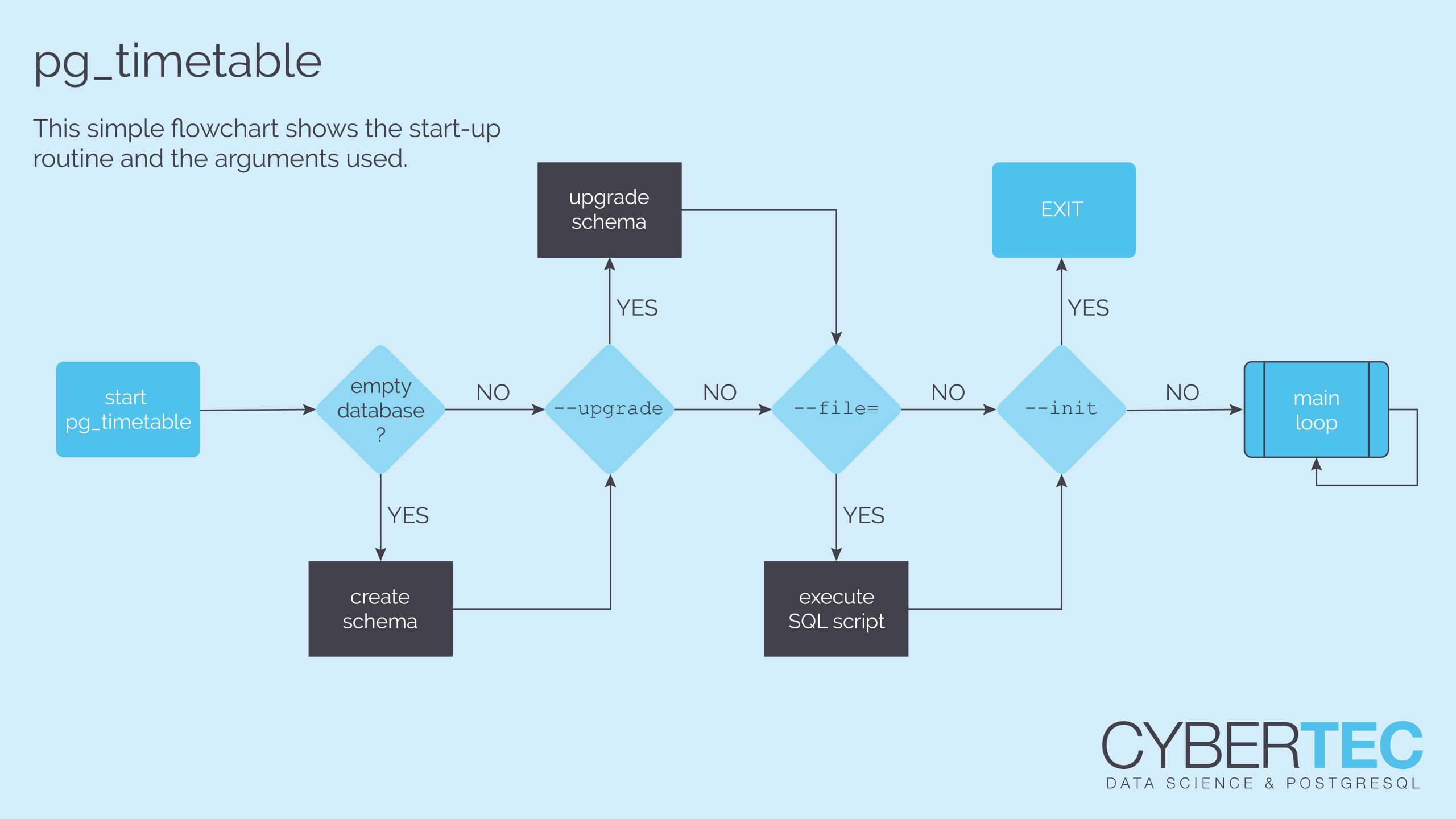
--init pg_timetable command-line argument--init command-line argument, if specified, will force pg_timetable to create the database schema and exit immediately.
During start-up, the database schema is created automatically if absent. Later a worker proceeds into the main loop checking chains and executing tasks.
This behavior is stable, however, mostly unusable in automation scenarios. Usually, you split preparation and work into separate stages. Now you can automate your scripts not only init pg_timetable environment but upgrade it as well. Consider this:
|
1 |
$ pg_timetable -c worker01 --init --upgrade postgresql://foo@bar/baz |
--file pg_timetable command-line argumentThat's not all! After schema initialization, one usually wants to add some tasks and chains. Either you are debugging your environment or deploying into production, there are traditionally prepared tasks you want to put into work. In previous versions, one should execute an additional step for that. But we've added --file command-line argument. You can now specify SQL script to be executed, not only during initialization or upgrade, but during an everyday routine.
--no-help pg_timetable command-line argumentIf you want more control over output, you may use --no-help command-line argument. The reason might be the same. Pretend you're using pg_timetable in some script, and the only thing you need to know is an exit code. But pg_timetable often tries to provide users with hints about why termination occurred. To suppress help messages, add this command-line argument.
If you start pg_timetable with only parameters needed and a clean database, it will create the necessary schema and proceed into the main loop. Below you can see a typical output. As you can see no tasks available.
|
1 2 3 4 5 6 7 8 9 10 11 12 13 14 15 16 17 18 19 20 21 22 23 |
$ pg_timetable -c worker01 postgresql://scheduler@localhost/timetable [ 2020-06-25 12:16:09.744 | LOG ]: Connection established... [ 2020-06-25 12:16:09.800 | LOG ]: Proceeding as 'worker01' with client PID 15668 [ 2020-06-25 12:16:09.801 | LOG ]: Executing script: DDL [ 2020-06-25 12:16:09.898 | LOG ]: Schema file executed: DDL [ 2020-06-25 12:16:09.905 | LOG ]: Executing script: JSON Schema [ 2020-06-25 12:16:09.909 | LOG ]: Schema file executed: JSON Schema [ 2020-06-25 12:16:09.910 | LOG ]: Executing script: Built-in Tasks [ 2020-06-25 12:16:09.911 | LOG ]: Schema file executed: Built-in Tasks [ 2020-06-25 12:16:09.913 | LOG ]: Executing script: Job Functions [ 2020-06-25 12:16:09.917 | LOG ]: Schema file executed: Job Functions [ 2020-06-25 12:16:09.917 | LOG ]: Configuration schema created... [ 2020-06-25 12:16:09.954 | LOG ]: Checking for @reboot task chains... [ 2020-06-25 12:16:09.957 | LOG ]: Number of chains to be executed: 0 [ 2020-06-25 12:16:09.958 | LOG ]: Checking for task chains... [ 2020-06-25 12:16:09.958 | LOG ]: Checking for interval task chains... [ 2020-06-25 12:16:09.960 | LOG ]: Number of chains to be executed: 0 [ 2020-06-25 12:16:09.993 | LOG ]: Number of active interval chains: 0 [ 2020-06-25 12:17:09.958 | LOG ]: Checking for task chains... [ 2020-06-25 12:17:09.958 | LOG ]: Checking for interval task chains... [ 2020-06-25 12:17:09.960 | LOG ]: Number of chains to be executed: 0 [ 2020-06-25 12:17:09.993 | LOG ]: Number of active interval chains: 0 ... |
Create schema if needed and exit returning 0 code. Can be combined with --upgrade argument, if new version of pg_timetable supposed to be run against old schema.
|
1 2 3 4 5 6 7 8 9 10 11 12 13 14 15 16 |
$ pg_timetable -c worker01 --init postgresql://scheduler@localhost/timetable [ 2020-06-25 12:33:04.232 | LOG ]: Connection established... [ 2020-06-25 12:33:04.285 | LOG ]: Proceeding as 'worker01' with client PID 9684 [ 2020-06-25 12:33:04.286 | LOG ]: Executing script: DDL [ 2020-06-25 12:33:04.385 | LOG ]: Schema file executed: DDL [ 2020-06-25 12:33:04.401 | LOG ]: Executing script: JSON Schema [ 2020-06-25 12:33:04.405 | LOG ]: Schema file executed: JSON Schema [ 2020-06-25 12:33:04.406 | LOG ]: Executing script: Built-in Tasks [ 2020-06-25 12:33:04.407 | LOG ]: Schema file executed: Built-in Tasks [ 2020-06-25 12:33:04.409 | LOG ]: Executing script: Job Functions [ 2020-06-25 12:33:04.410 | LOG ]: Schema file executed: Job Functions [ 2020-06-25 12:33:04.413 | LOG ]: Configuration schema created... [ 2020-06-25 12:33:04.413 | LOG ]: Closing session $ echo $? 0 |
You may specify arbitrary SQL script to execute during start-up. But beware you are not duplicating tasks in case of a working system. Here I will add sample chain and pg_timetable will execute it in the main loop when the time has come.
|
1 2 3 4 5 6 7 8 9 10 11 12 13 14 15 16 17 18 19 20 21 22 23 |
$ pg_timetable -c worker01 --file='samples/basic.sql' postgresql://scheduler@localhost/timetable [ 2020-06-25 12:41:59.661 | LOG ]: Connection established... [ 2020-06-25 12:41:59.712 | LOG ]: Proceeding as 'worker01' with client PID 7964 [ 2020-06-25 12:41:59.713 | LOG ]: Executing script: DDL [ 2020-06-25 12:41:59.801 | LOG ]: Schema file executed: DDL [ 2020-06-25 12:41:59.812 | LOG ]: Executing script: JSON Schema [ 2020-06-25 12:41:59.814 | LOG ]: Schema file executed: JSON Schema [ 2020-06-25 12:41:59.816 | LOG ]: Executing script: Built-in Tasks [ 2020-06-25 12:41:59.817 | LOG ]: Schema file executed: Built-in Tasks [ 2020-06-25 12:41:59.818 | LOG ]: Executing script: Job Functions [ 2020-06-25 12:41:59.819 | LOG ]: Schema file executed: Job Functions [ 2020-06-25 12:41:59.822 | LOG ]: Configuration schema created... [ 2020-06-25 12:41:59.823 | LOG ]: Executing script: samples/basic.sql [ 2020-06-25 12:41:59.824 | LOG ]: Script file executed: samples/basic.sql [ 2020-06-25 12:41:59.862 | LOG ]: Checking for @reboot task chains... [ 2020-06-25 12:41:59.867 | LOG ]: Number of chains to be executed: 0 [ 2020-06-25 12:41:59.867 | LOG ]: Checking for task chains... [ 2020-06-25 12:41:59.868 | LOG ]: Checking for interval task chains... [ 2020-06-25 12:41:59.871 | LOG ]: Number of chains to be executed: 1 [ 2020-06-25 12:41:59.875 | LOG ]: Starting chain ID: 1; configuration ID: 1 [ 2020-06-25 12:41:59.905 | LOG ]: Number of active interval chains: 0 [ 2020-06-25 12:41:59.920 | LOG ]: Executed successfully chain ID: 1; configuration ID: 1 ... |
The same example on existing schema adding some interval chains. As you can see, no schema is created this time, but the custom script is executed either way.
|
1 2 3 4 5 6 7 8 9 10 11 12 13 14 15 16 17 18 |
$ pg_timetable -c worker01 --file='samples/interval.sql' postgresql://scheduler@localhost/timetable [ 2020-06-25 12:48:07.300 | LOG ]: Connection established... [ 2020-06-25 12:48:07.360 | LOG ]: Proceeding as 'worker01' with client PID 8840 [ 2020-06-25 12:48:07.363 | LOG ]: Executing script: samples/interval.sql [ 2020-06-25 12:48:07.374 | LOG ]: Script file executed: samples/interval.sql [ 2020-06-25 12:48:07.411 | LOG ]: Checking for @reboot task chains... [ 2020-06-25 12:48:07.414 | LOG ]: Number of chains to be executed: 0 [ 2020-06-25 12:48:07.415 | LOG ]: Checking for task chains... [ 2020-06-25 12:48:07.416 | LOG ]: Checking for interval task chains... [ 2020-06-25 12:48:07.419 | LOG ]: Number of chains to be executed: 1 [ 2020-06-25 12:48:07.423 | LOG ]: Starting chain ID: 1; configuration ID: 1 [ 2020-06-25 12:48:07.454 | LOG ]: Number of active interval chains: 2 [ 2020-06-25 12:48:07.456 | LOG ]: Starting chain ID: 2; configuration ID: 3 [ 2020-06-25 12:48:07.466 | LOG ]: Executed successfully chain ID: 1; configuration ID: 1 [ 2020-06-25 12:48:07.494 | LOG ]: Starting chain ID: 2; configuration ID: 2 [ 2020-06-25 12:48:07.500 | USER ]: Severity: NOTICE; Message: Sleeping for 5 sec in Configuration @after 10 seconds [ 2020-06-25 12:48:07.512 | USER ]: Severity: NOTICE; Message: Sleeping for 5 sec in Configuration @every 10 seconds ... |
Suppose we want to upgrade pg_timetable version, but with that we want clean logs for the new version. In this case, one may start it in --upgrade mode, provide special actions to be done with --file="backup_logs.sql" and specify --init to exit immediately after upgrade.
|
1 2 3 4 5 6 7 8 9 10 11 12 13 14 15 16 17 18 19 20 |
$ cat backup_logs.sql CREATE TABLE timetable.log_backup AS SELECT * FROM timetable.log; TRUNCATE timetable.log; $ pg_timetable -c worker01 --init --upgrade --file='backup_logs.sql' postgresql://scheduler@localhost/timetable [ 2020-06-25 13:22:16.161 | LOG ]: Connection established... [ 2020-06-25 13:22:16.215 | LOG ]: Proceeding as 'worker01' with client PID 16652 [ 2020-06-25 13:22:16.220 | LOG ]: Executing script: backup_logs.sql [ 2020-06-25 13:22:16.250 | LOG ]: Script file executed: backup_logs.sql [ 2020-06-25 13:22:16.251 | LOG ]: Upgrading database... [ 2020-06-25 13:22:16.255 | USER ]: Severity: NOTICE; Message: relation 'migrations' already exists, skipping [ 2020-06-25 13:22:16.255 | LOG ]: Closing session $ psql -U scheduler -d timetable -c 'dt timetable.log*' List of relations Schema | Name | Type | Owner -----------+------------+-------+----------- timetable | log | table | scheduler timetable | log_backup | table | scheduler (2 rows) |
|
1 2 3 4 5 6 7 8 9 10 11 12 13 14 15 16 17 18 19 20 21 22 23 24 25 26 27 28 29 |
$ pg_timetable the required flag `-c, --clientname' was not specified Usage: pg_timetable Application Options: -c, --clientname= Unique name for application instance -v, --verbose Show verbose debug information [$PGTT_VERBOSE] -h, --host= PG config DB host (default: localhost) [$PGTT_PGHOST] -p, --port= PG config DB port (default: 5432) [$PGTT_PGPORT] -d, --dbname= PG config DB dbname (default: timetable) [$PGTT_PGDATABASE] -u, --user= PG config DB user (default: scheduler) [$PGTT_PGUSER] -f, --file= SQL script file to execute during startup --password= PG config DB password (default: somestrong) [$PGTT_PGPASSWORD] --sslmode=[disable|require] What SSL priority use for connection (default: disable) --pgurl= PG config DB url [$PGTT_URL] --init Initialize database schema and exit. Can be used with --upgrade --upgrade Upgrade database to the latest version --no-shell-tasks Disable executing of shell tasks [$PGTT_NOSHELLTASKS] [ 2020-06-25 12:57:59.122 | PANIC ]: Error parsing command line arguments: the required flag `-c, --clientname' was not specified $ echo $? 2 $ pg_timetable --no-help the required flag `-c, --clientname' was not specified $ echo $? 2 |
If you want to know about every improvement and a bug fix in the previous version, please, check our repository Release page.
And do not forget to Star it, Watch it and maybe even Fork it. Why not? We are Open Source after all!
Stay safe! Love! Peace! Elephant! ❤??
UPDATED 08.05.2023 - SQL and especially PostgreSQL provide a nice set of general purpose data types you can use to model your data. However, what if you want to store fewer generic data? What if you want to have more advanced server-side check constraints? The way to do that in SQL and in PostgreSQL in particular is to use CREATE DOMAIN.
This blog will show you how to create useful new data types with constraints for:
These are all commonly needed in many applications.
The first example is about color codes. As you can see, not every string is a valid color code, so you must add restrictions. Here are some examples of valid color codes: #00ccff, #039, ffffcc.
|
1 2 3 4 5 6 7 8 9 10 11 12 13 14 15 |
test=# h CREATE DOMAIN Command: CREATE DOMAIN Description: define a new domain Syntax: CREATE DOMAIN name [ AS ] data_type [ COLLATE collation ] [ DEFAULT expression ] [ constraint [ ... ] ] where constraint is: [ CONSTRAINT constraint_name ] { NOT NULL | NULL | CHECK (expression) } URL: https://www.postgresql.org/docs/15/sql-createdomain.html |
What CREATE DOMAIN really does is to abstract a data type and to add constraints. The new domain can then be used just like all other data types (varchar, integer, boolean, etc). Let's take a look and see how it works:
|
1 2 |
CREATE DOMAIN color_code AS text CHECK (VALUE ~ '^#?([a-f]|[A-F]|[0-9]){3}(([a-f]|[A-F]|[0-9]){3})? |
What you do here is to assign a regular expression to the color code. Every time you use a color code, PostgreSQL will check the expression and throw an error in case the value does not match the constraint. Let's take a look at a real example:
|
1 2 |
test=# CREATE TABLE t_demo (c color_code); CREATE TABLE |
You can see that the domain used is a standard column type. Let's insert a value:
|
1 2 |
test=# INSERT INTO t_demo VALUES ('#04a'); INSERT 0 1 |
The value matches the constraint, therefore everything is OK. However, if you try to add an incorrect input value, PostgreSQL will complain instantly:
|
1 2 |
test=# INSERT INTO t_demo VALUES ('#04XX'); ERROR: value for domain color_code violates check constraint 'color_code_check' |
The CHECK constraint will prevent the insertion from happening.
More often than not, you'll need alphanumeric strings. Maybe you want to store an identifier, or a voucher code. Alphanumeric strings are quite common and really useful. Here's how it works:
|
1 2 |
CREATE DOMAIN alphanumeric_string AS text CHECK (VALUE ~ '[a-z0-9].*'); |
The regular expression is pretty simple in this case. You need to decide if you want to accept upper-case or only lower-case letters. PostgreSQL offers case-sensitive and case-insensitive regular expression operators.
Imagine you want to check if a password is strong enough. A domain can help in this case as well:
|
1 2 3 4 5 |
-- password: Should have 1 lowercase letter, 1 uppercase letter, 1 number, -- 1 special character and be at least 8 characters long CREATE DOMAIN password_text AS text CHECK (VALUE ~ '(?=(.*[0-9]))(?=.*[!@#$%^&*()\[]{}-_+=~`|:;'''<>,./?])(?=.*[a-z])(?=(.*[A-Z])) (?=(.*)).{8,}'); |
This expression is a bit more complicated, but there's no need to understand it. Just copy and paste it and you'll be fine. Also: This expression is here to verify data - it is not an invitation to store plain text passwords in the database.
If you want to store URLs and if you want to make sure that the format is correct, you can also make use of CREATE DOMAIN. The following snippet shows how you can verify an URL:
|
1 2 |
CREATE DOMAIN url AS text CHECK (VALUE ~ '^https?://[-a-zA-Z0-9@:%._+~#=]{2,255}.[a-z]{2,6}(/[-a-zA-Z0-9@:%._+~#=]*)*(?[-a-zA-Z0-9@:%_+.~#()?&//=]*)? |
If you want to match a domain name only, the following expression will do:
|
1 2 3 |
-- domains CREATE DOMAIN domain AS text CHECK (VALUE ~ '^([a-z][a-z0-9-]+(.|-*.))+[a-z]{2,6} |
People often ask if a domain has performance implications. Basically, all the domain does is to enforce a constraint - the underlying data type is still the same, and therefore there's not much of a difference between adding a CHECK constraint for every column. The real benefit of a domain is not better performance - it's data type abstraction. Abstraction is what you would do in any high-level language.
CREATE DOMAIN isn't the only cool feature in PostgreSQL. If you want to know more about regular expressions in PostgreSQL, I suggest checking out my blog post about how to match “Gadaffi” which is more complicated than it might look at first glance.