Users with an Oracle background consider tablespaces very important and are surprised that you can find so little information about them in PostgreSQL. This article will explain what they are, when they are useful and whether or not you should use them.
Essentially, a tablespace in PostgreSQL is a directory containing data files. These data files are the storage behind objects with a state: tables, sequences, indexes and materialized views. In PostgreSQL, each such object has its own data file. If the object is bigger, it will have several files called segments with a size limit of 1GB.
PostgreSQL uses the operating system's file system for its storage. This is different from Oracle, which essentially implements its own “file system”.
Let's compare the terms for clarity:
| Oracle | PostgreSQL or operating system |
|---|---|
| tablespace | file system |
| datafile | logical/physical volume |
| segment | all data files of a table |
| extent | segment / data file |
Each PostgreSQL database cluster initially has two tablespaces. You can list them with db in psql:
|
1 2 3 4 5 6 |
List of tablespaces Name | Owner | Location ------------+----------+---------- pg_default | postgres | pg_global | postgres | (2 rows) |
You'll notice that there is no location specified. That is because they always correspond to fixed subdirectories of the PostgreSQL data directory: the default tablespace (pg_default) is the “base” subdirectory, and the global tablespace (pg_global) is the “global” subdirectory.
By default, all data files will be stored in the default tablespace. Only certain objects are stored in the global tablespace: the catalog tables pg_database, pg_authid, pg_tablespace and pg_shdepend and all their indexes. These are the only catalog tables shared by all databases.
To create a new tablespace, you first have to create a new directory. Don't create that directory in the PostgreSQL data directory!
Note that the directory has to belong to the “postgres” operating system user (to be exact, the user has to have permissions to change the directory's permissions).
Then you can create the tablespace:
|
1 |
CREATE TABLESPACE mytbsp LOCATION '/tmp/mytbsp'; |
To use the tablespace, you can create a table or another object with storage in it:
|
1 2 3 4 5 6 7 8 9 10 11 |
CREATE TABLE newtab ( id integer NOT NULL, val text NOT NULL ) TABLESPACE mytbsp; ALTER TABLE newtab ADD CONSTRAINT newtab_pkey PRIMARY KEY (id) USING INDEX TABLESPACE mytbsp; CREATE INDEX newtab_val_idx ON newtab (val) TABLESPACE mytbsp; |
Note that indexes are not automatically created in the same tablespace as the table.
You can also create a database in a tablespace:
|
1 |
CREATE DATABASE newdb TABLESPACE mytbsp; |
Then all objects you create in that database will automatically be placed in the database's tablespace.
There are ALTER commands to change the tablespace of any object. Moving an object to another tablespace copies the data files, and the object is inaccessible while it is being moved.
If you perform a file system backup of a database with tablespaces, you have to back up all tablespaces. You cannot back up or restore a single tablespace, and there is no equivalent to Oracle's “transportable tablespaces”.
pg_basebackup with the plain format will try to save tablespaces in the same place as on the database server (the -D option only specifies the location of the data directory). To backup data from a tablespace to a different location, you have to use the option --tablespace-mapping=olddir=newdir. You can use this option more than once for multiple tablespaces.
Using tablespaces makes database administration more complicated, because the data directory no longer contains all the data.
In the vast majority of cases, you shouldn't create extra tablespaces in PostgreSQL. In particular, it never makes sense to create a tablespace on the same file system as the data directory or on the same file system as another tablespace.
So what are the benefits of tablespaces that justify the administrative complexity?
seq_page_cost, random_page_cost and effective_io_concurrency options on the tablespace to tell the optimizer about the performance characteristics.temp_tablespaces parameter to a different tablespace.If you are running in a virtualized environment with virtualized storage, all these points are moot, with the exception of the third. Since almost everybody uses virtualization these days, tablespaces are becoming an increasingly irrelevant PostgreSQL feature.
There is a tenacious myth circulating among database administrators that you should put tables and indexes on different disks for good performance.
You will hear people making elaborate arguments as to why the particular interplay of access patterns during an index scan will make this efficient on spinning disks. But spinning disks are going out of business, and you typically only saturate your storage system with several concurrent SQL statements, when all such access patterns will be disrupted anyway.
The truth behind the myth is that it is certainly beneficial to spread the I/O load over multiple devices. If you use striping on the operating system level, you will get a better spread than you will by carefully placing tables and indexes.
Tablespaces are rarely relevant in PostgreSQL. Resist the temptation to create tablespaces and leave all data in the default tablespace.
Just like any advanced relational database, PostgreSQL uses a cost-based query optimizer that tries to turn your SQL queries into something efficient that executes in as little time as possible. For many people, the workings of the optimizer itself remain a mystery, so we have decided to give users some insight into what is really going on behind the scenes.
So let’s take a tour through the PostgreSQL optimizer and get an overview of some of the most important techniques the optimizer uses to speed up queries. Note that the techniques listed here are in no way complete. There is a lot more going on, but it makes sense to take a look at the most basic things in order to gain a good understanding of the process.
Constant folding is one of the easier processes to understand. Nonetheless, it's extremely important.
|
1 2 3 4 5 6 7 8 9 10 11 12 13 14 15 16 |
demo=# SELECT * FROM generate_series(1, 10) AS x WHERE x = 7 + 1; x --- 8 (1 row) demo=# explain SELECT * FROM generate_series(1, 10) AS x WHERE x = 7 + 1; QUERY PLAN ---------------------------------------------------------------------- Function Scan on generate_series x (cost=0.00..0.13 rows=1 width=4) Filter: (x = 8) (2 rows) |
Here we add a filter to the query: x = 7 + 1. What the system does is to “fold” the constant and instead do “x = 8”. Why is that important? In case “x” is indexed (assuming it is a table), we can easily look up 8 in the index.
|
1 2 3 4 5 6 7 8 |
demo=# explain SELECT * FROM generate_series(1, 10) AS x WHERE x - 1 = 7 ; QUERY PLAN ---------------------------------------------------------------------- Function Scan on generate_series x (cost=0.00..0.15 rows=1 width=4) Filter: ((x - 1) = 7) (2 rows) |
PostgreSQL does not transform the expression to “x = 8” in this case. That’s why you should try to make sure that the filter is on the right side, and not on the column you might want to index.
One more important technique is the idea of function inlining. The goal is to reduce function calls as much as possible and thus speed up the query.
|
1 2 3 4 5 6 7 8 9 10 11 12 |
demo=# CREATE OR REPLACE FUNCTION ld(int) RETURNS numeric AS $ SELECT log(2, $1); $ LANGUAGE 'sql'; CREATE FUNCTION demo=# SELECT ld(1024); ld --------------------- 10.0000000000000000 (1 row) |
2^10 = 1024. This looks right.
|
1 2 3 4 5 6 7 8 |
demo=# explain SELECT * FROM generate_series(1, 10) AS x WHERE ld(x) = 1000; QUERY PLAN ---------------------------------------------------------------------- Function Scan on generate_series x (cost=0.00..0.18 rows=1 width=4) Filter: (log('2'::numeric, (x)::numeric) = '1000'::numeric) (2 rows) |
Look in the WHERE clause. The ld function has been replaced with the underlying log function. Note that this is only possible in the case of SQL functions. PL/pgSQL and other stored procedure languages are black boxes to the optimizer, so whether these things are possible or not depends on the type of language used.
|
1 2 3 4 5 6 7 8 9 10 11 12 13 14 15 16 |
demo=# CREATE OR REPLACE FUNCTION pl_ld(int) RETURNS numeric AS $ BEGIN RETURN log(2, $1); END; $ LANGUAGE 'plpgsql'; CREATE FUNCTION demo=# explain SELECT * FROM generate_series(1, 10) AS x WHERE pl_ld(x) = 1000; QUERY PLAN ---------------------------------------------------------------------- Function Scan on generate_series x (cost=0.00..2.63 rows=1 width=4) Filter: (pl_ld(x) = '1000'::numeric) (2 rows) |
In this case, inlining is not possible. While the code is basically the same, the programming language does make a major difference.
Something that is often overlooked is the concept of function stability. When creating a function, it makes a difference if a function is created as VOLATILE (default), STABLE, or as IMMUTABLE. It can even make a major difference - especially if you are using indexes. Let’s create some sample data and sort these differences out:
VOLATILE means that a function is not guaranteed to return the same result within the same transaction given the same input parameters. In other words, the PostgreSQL optimizer cannot see the function as a constant, and has to execute it for every row.
|
1 2 3 4 5 6 7 |
demo=# CREATE TABLE t_date AS SELECT * FROM generate_series('1900-01-01'::timestamptz, '2021-12-31'::timestamptz, '1 minute') AS x; SELECT 64164961 demo=# CREATE INDEX idx_date ON t_date (x); CREATE INDEX |
We have generated a list of 64 million entries containing 1 row per minute since January 1900, which produces 64 million entries.
VOLATILE function:|
1 2 3 4 5 6 7 8 9 10 11 12 13 14 15 16 17 |
demo=# explain analyze SELECT * FROM t_date WHERE x = clock_timestamp(); QUERY PLAN ------------------------------------------------------------------- Gather (cost=1000.00..685947.45 rows=1 width=8) (actual time=2656.961..2658.547 rows=0 loops=1) Workers Planned: 2 Workers Launched: 2 -> Parallel Seq Scan on t_date (cost=0.00..684947.35 rows=1 width=8) (actual time=2653.009..2653.009 rows=0 loops=3) Filter: (x = clock_timestamp()) Rows Removed by Filter: 21388320 Planning Time: 0.056 ms Execution Time: 2658.562 ms (8 rows) |
In this case, the query needs a whopping 2.6 seconds and eats up a ton of resources. The reason is that clock_timestamp() is VOLATILE.
STABLE function?|
1 2 3 4 5 6 7 8 9 10 11 12 13 |
demo=# explain analyze SELECT * FROM t_date WHERE x = now(); QUERY PLAN --------------------------------------------------------------- Index Only Scan using idx_date on t_date (cost=0.57..4.59 rows=1 width=8) (actual time=0.014..0.015 rows=0 loops=1) Index Cond: (x = now()) Heap Fetches: 0 Planning Time: 0.060 ms Execution Time: 0.026 ms (5 rows) |
The query is many thousands of times faster, because now PostgreSQL can turn it into a constant and thus use the index. If you want to learn more about function stability in PostgreSQL, here is more information.
The next optimization on our list is the concept of equality constraints. What PostgreSQL tries to do here is to derive implicit knowledge about the query.
|
1 2 3 4 5 6 7 8 9 10 11 12 13 |
demo=# CREATE TABLE t_demo AS SELECT x, x AS y FROM generate_series(1, 1000) AS x; SELECT 1000 demo=# SELECT * FROM t_demo LIMIT 5; x | y ---+--- 1 | 1 2 | 2 3 | 3 4 | 4 5 | 5 (5 rows) |
|
1 2 3 4 5 6 7 8 9 |
demo=# explain SELECT * FROM t_demo WHERE x = y AND y = 4; QUERY PLAN ------------------------------------------------------- Seq Scan on t_demo (cost=0.00..20.00 rows=1 width=8) Filter: ((x = 4) AND (y = 4)) (2 rows) |
Again, the magic is in the execution plan. You can see that PostgreSQL has figured that x and y are 4.
|
1 2 3 4 5 6 7 8 9 10 11 12 |
demo=# CREATE INDEX idx_x ON t_demo (x); CREATE INDEX demo=# explain SELECT * FROM t_demo WHERE x = y AND y = 4; QUERY PLAN -------------------------------------------------------------------- Index Scan using idx_x on t_demo (cost=0.28..8.29 rows=1 width=8) Index Cond: (x = 4) Filter: (y = 4) (3 rows) |
Without this optimization, it would be absolutely impossible to use the index we have just created. In order to optimize the query, PostgreSQL will automatically figure out that we can use an index here.
Indexes are important!
When talking about the PostgreSQL optimizer and query optimization there is no way to ignore views and subselect handling.
|
1 2 3 4 5 6 7 8 9 10 11 12 13 14 |
demo=# CREATE VIEW v1 AS SELECT * FROM generate_series(1, 10) AS x; CREATE VIEW demo=# explain SELECT * FROM v1 ORDER BY x DESC; QUERY PLAN ---------------------------------------------- Sort (cost=0.27..0.29 rows=10 width=4) Sort Key: x.x DESC -> Function Scan on generate_series x (cost=0.00..0.10 rows=10 width=4) (3 rows) |
When we look at the execution plan, the view is nowhere to be seen.
|
1 2 3 |
SELECT * FROM v1 ORDER BY x DESC; |
|
1 2 3 4 5 |
SELECT * FROM (SELECT * FROM generate_series(1, 10) AS x ) AS v1 ORDER BY x DESC; |
|
1 2 3 |
SELECT * FROM generate_series(1, 10) AS x ORDER BY x DESC; |
from_collapse_limit, which controls this behavior:|
1 2 3 4 5 |
demo=# SHOW from_collapse_limit; from_collapse_limit --------------------- 8 (1 row) |
The meaning of this parameter is that only up to 8 subselects in the FROM clause will be flattened out. If there are more than 8 subselects, they will be executed without being flattened out. In most real-world use cases, this is not a problem. It can only become an issue if the SQL statements used are very complex. More information about joins and join_collapse_limit can be found in our blog.
Keep in mind that inlining is not always possible. Developers are aware of that.
Joins are used in most queries and are therefore of incredible importance to good performance. We’ll now focus on some of the techniques relevant to joins in general.
The next important thing on our list is the way the PostgreSQL optimizer handles join orders. In a PostgreSQL database, joins are not necessarily done in the order proposed by the end user - quite the opposite: The query optimizer tries to figure out as many join options as possible.
|
1 2 3 4 5 6 7 8 9 10 11 12 13 14 15 |
demo=# CREATE TABLE a AS SELECT x, x % 10 AS y FROM generate_series(1, 100000) AS x ORDER BY random(); SELECT 100000 demo=# CREATE TABLE b AS SELECT x, x % 10 AS y FROM generate_series(1, 1000000) AS x ORDER BY random(); SELECT 1000000 demo=# CREATE TABLE c AS SELECT x, x % 10 AS y FROM generate_series(1, 10000000) AS x ORDER BY random(); SELECT 10000000 |
|
1 2 3 4 5 6 7 8 |
demo=# CREATE INDEX a_x ON a(x); CREATE INDEX demo=# CREATE INDEX b_x ON b(x); CREATE INDEX demo=# CREATE INDEX c_x ON c(x); CREATE INDEX demo=# ANALYZE; ANALYZE |
|
1 2 3 4 5 6 7 8 9 10 11 12 13 14 15 16 17 18 19 |
demo=# explain SELECT * FROM a, b, c WHERE c.x = a.x AND a.x = b.x AND a.x = 10; QUERY PLAN -------------------------------------------------------------------- Nested Loop (cost=1.15..25.23 rows=1 width=24) -> Nested Loop (cost=0.72..16.76 rows=1 width=16) -> Index Scan using a_x on a (cost=0.29..8.31 rows=1 width=8) Index Cond: (x = 10) -> Index Scan using b_x on b (cost=0.42..8.44 rows=1 width=8) Index Cond: (x = 10) -> Index Scan using c_x on c (cost=0.43..8.45 rows=1 width=8) Index Cond: (x = 10) (8 rows) |
Note that the query joins “c and a” and then “a and b”. However, let’s look at the plan more closely. PostgreSQL starts with index scans on a and b. The result is then joined with c. Three indexes are used. This happens because of the equality constraints we discussed before. To find out about forcing the join order, see this blog.
Many people keep asking about explicit versus implicit joins. Basically, both variants are the same.
|
1 2 3 |
SELECT * FROM a, b WHERE a.id = b.id; vs. SELECT * FROM a JOIN b ON a.id = b.id; |
Both queries are identical and the planner will treat them the same way for most commonly seen queries. Mind that the explicit joins work with and without parenthesis.
join_collapse_limit:|
1 2 3 4 5 |
demo=# SHOW join_collapse_limit; join_collapse_limit --------------------- 8 (1 row) |
The join_collapse_limit parameter controls how many explicit joins are planned implicitly. In other words, an implicit join is just like an explicit join, but only up to a certain number of joins controlled by this parameter. See this blog for more information. It is also possible to use join_collapse_limit to force the join order, as explained in this blog.
For the sake of simplicity, we can assume that it makes no difference for 95% of all queries and for most customers.
PostgreSQL offers various join strategies. These strategies include hash joins, merge joins, nested loops, and a lot more. We have already shared some of this information in previous posts. More on PostgreSQL join strategies can be found here.
Optimizing outer joins (LEFT JOIN, RIGHT JOIN, etc.) is an important topic. Usually, the planner has fewer options here than in the case of inner joins. The following optimizations are possible:
|
1 2 |
(A leftjoin B on (Pab)) innerjoin C on (Pac) = (A innerjoin C on (Pac)) leftjoin B on (Pab) |
where Pac is a predicate referencing A and C, etc (in this case, clearly
Pac cannot reference B, or the transformation is nonsensical).
|
1 2 3 4 5 |
(A leftjoin B on (Pab)) leftjoin C on (Pac) = (A leftjoin C on (Pac)) leftjoin B on (Pab) (A leftjoin B on (Pab)) leftjoin C on (Pbc) = A leftjoin (B leftjoin C on (Pbc)) on (Pab) |
While this theoretical explanation is correct, most people will have no clue what it means in real life.
|
1 2 3 4 5 6 7 8 9 10 11 12 13 14 15 16 17 18 19 20 21 22 |
demo=# explain SELECT * FROM generate_series(1, 10) AS x LEFT JOIN generate_series(1, 100) AS y ON (x = y) JOIN generate_series(1, 10000) AS z ON (y = z) ; QUERY PLAN -------------------------------------------------------------------- Hash Join (cost=1.83..144.33 rows=500 width=12) Hash Cond: (z.z = x.x) -> Function Scan on generate_series z (cost=0.00..100.00 rows=10000 width=4) -> Hash (cost=1.71..1.71 rows=10 width=8) -> Hash Join (cost=0.23..1.71 rows=10 width=8) Hash Cond: (y.y = x.x) -> Function Scan on generate_series y (cost=0.00..1.00 rows=100 width=4) -> Hash (cost=0.10..0.10 rows=10 width=4) -> Function Scan on generate_series x (cost=0.00..0.10 rows=10 width=4) (9 rows) |
What we see here is that the PostgreSQL optimizer decides on joining x with y and then with z. In other words, the PostgreSQL optimizer has simply followed the join order as used in the SQL statement.
|
1 2 3 4 5 6 7 8 9 10 11 12 13 14 15 16 17 18 19 20 21 22 |
demo=# explain SELECT * FROM generate_series(1, 10) AS x LEFT JOIN generate_series(1, 100000) AS y ON (x = y) JOIN generate_series(1, 100) AS z ON (y = z) ; QUERY PLAN -------------------------------------------------------------------- Hash Join (cost=1.83..1426.83 rows=5000 width=12) Hash Cond: (y.y = x.x) -> Function Scan on generate_series y (cost=0.00..1000.00 rows=100000 width=4) -> Hash (cost=1.71..1.71 rows=10 width=8) -> Hash Join (cost=0.23..1.71 rows=10 width=8) Hash Cond: (z.z = x.x) -> Function Scan on generate_series z (cost=0.00..1.00 rows=100 width=4) -> Hash (cost=0.10..0.10 rows=10 width=4) -> Function Scan on generate_series x (cost=0.00..0.10 rows=10 width=4) (9 rows) |
The difference is that PostgreSQL again starts with x but then joins z first, before adding y.
Note that this optimization happens automatically. One reason why the optimizer can make this decision is because of the existence of optimizer support functions which were added to PostgreSQL a while ago. The reason why the reordering works is that support functions offer the planner a chance to figure out how many rows are returned from which part. If you use tables instead of set returning functions, support functions are irrelevant. PostgreSQL v16 has added support for "anti-joins" in RIGHT and OUTER queries.
Not every join in a query is actually executed by PostgreSQL. The optimizer knows the concept of join pruning and is able to get rid of pointless joins quite efficiently. The main question is: When is that possible, and how can we figure out what’s going on?
The next listing shows how some suitable sample data can be created:
|
1 2 3 4 5 6 7 8 9 10 |
demo=# CREATE TABLE t_left AS SELECT * FROM generate_series(1, 1000) AS id; SELECT 1000 demo=# CREATE UNIQUE INDEX idx_left ON t_left (id); CREATE INDEX demo=# CREATE TABLE t_right AS SELECT * FROM generate_series(1, 100) AS id; SELECT 100 demo=# CREATE UNIQUE INDEX idx_right ON t_right (id); CREATE INDEX |
|
1 2 3 4 5 6 7 8 9 10 11 12 13 14 15 |
demo=# d t_left Table 'public.t_left' Column | Type | Collation | Nullable | Default --------+---------+-----------+----------+--------- id | integer | | | Indexes: 'idx_left' UNIQUE, btree (id) demo=# d t_right Table 'public.t_right' Column | Type | Collation | Nullable | Default --------+---------+-----------+----------+--------- id | integer | | | Indexes: 'idx_right' UNIQUE, btree (id) |
|
1 2 3 4 5 6 7 8 9 10 11 |
demo=# explain SELECT * FROM t_left AS a LEFT JOIN t_right AS b ON (a.id = b.id); QUERY PLAN -------------------------------------------------------------------- Hash Left Join (cost=3.25..20.89 rows=1000 width=8) Hash Cond: (a.id = b.id) -> Seq Scan on t_left a (cost=0.00..15.00 rows=1000 width=4) -> Hash (cost=2.00..2.00 rows=100 width=4) -> Seq Scan on t_right b (cost=0.00..2.00 rows=100 width=4) (5 rows) |
In this case, the join has to be executed. As you can see, PostgreSQL has decided on a hash join.
|
1 2 3 4 5 6 7 |
demo=# explain SELECT a.* FROM t_left AS a LEFT JOIN t_right AS b ON (a.id = b.id); QUERY PLAN ------------------------------------------------------------ Seq Scan on t_left a (cost=0.00..15.00 rows=1000 width=4) (1 row) |
Join pruning can happen if we DO NOT read data from the right side, and if the right side is unique. If the right side is not unique, the join might actually increase the number of rows returned; so pruning is only possible in case the right side is unique.
|
1 2 3 4 5 6 7 8 9 10 11 12 13 14 |
demo=# DROP INDEX idx_right ; DROP INDEX demo=# explain SELECT a.* FROM t_left AS a LEFT JOIN t_right AS b ON (a.id = b.id); QUERY PLAN -------------------------------------------------------------------- Hash Left Join (cost=3.25..23.00 rows=1000 width=4) Hash Cond: (a.id = b.id) -> Seq Scan on t_left a (cost=0.00..15.00 rows=1000 width=4) -> Hash (cost=2.00..2.00 rows=100 width=4) -> Seq Scan on t_right b (cost=0.00..2.00 rows=100 width=4) (5 rows) |
While it is certainly a good thing to have join pruning in the PostgreSQL optimizer, you have to be aware of the fact that the planner is basically fixing something which should not exist anyway. Write queries efficiently in the first place; don’t add pointless joins.
There is also something common you will see everywhere in the code within SQL EXISTS. Here’s an example:
|
1 2 3 4 5 6 7 8 9 10 11 12 13 14 |
demo=# explain SELECT * FROM a WHERE NOT EXISTS (SELECT 1 FROM b WHERE a.x = b.x AND b.x = 42); QUERY PLAN ------------------------------------------------------------------- Hash Anti Join (cost=4.46..2709.95 rows=100000 width=8) Hash Cond: (a.x = b.x) -> Seq Scan on a (cost=0.00..1443.00 rows=100000 width=8) -> Hash (cost=4.44..4.44 rows=1 width=4) -> Index Only Scan using b_x on b (cost=0.42..4.44 rows=1 width=4) Index Cond: (x = 42) (6 rows) |
This might not look like a big deal, but consider the alternatives: What PostgreSQL does here is to create a “hash anti-join”. This is way more efficient than some sort of nested loop. In short: The nested loop is replaced with a join which can yield significant performance gains.
Every database relies heavily on sorting, which is necessary to handle many different types of queries and optimize various workloads. One of the key optimizations in this area is that PostgreSQL can use indexes to optimize ORDER BY in a very clever way. See more about how PostgreSQL can optimize subqueries in the blog Subqueries and Performance in PostgreSQL.
|
1 2 3 4 5 6 7 |
demo=# CREATE TABLE t_sample AS SELECT * FROM generate_series(1, 1000000) AS id ORDER BY random(); SELECT 1000000 demo=# VACUUM ANALYZE t_sample ; VACUUM |
The listing created a list of 1 million entries that’s been stored on disk in random order. Subsequently, VACUUM was called to ensure that all PostgreSQL hint bit-related issues were sorted out before the test is executed. If you want to know what hint bits are and how they operate, check out our post about hint bits in PostgreSQL.
|
1 2 3 4 5 6 7 8 9 10 11 12 13 14 15 16 17 18 19 20 21 22 23 24 |
demo=# explain analyze SELECT * FROM t_sample ORDER BY id DESC LIMIT 100; QUERY PLAN ------------------------------------------------------------------- Limit (cost=25516.40..25528.07 rows=100 width=4) (actual time=84.806..86.252 rows=100 loops=1) -> Gather Merge (cost=25516.40..122745.49 rows=833334 width=4) (actual time=84.805..86.232 rows=100 loops=1) Workers Planned: 2 Workers Launched: 2 -> Sort (cost=24516.38..25558.05 rows=416667 width=4) (actual time=65.576..65.586 rows=82 loops=3) Sort Key: id DESC Sort Method: top-N heapsort Memory: 33kB Worker 0: Sort Method: top-N heapsort Memory: 32kB Worker 1: Sort Method: top-N heapsort Memory: 33kB -> Parallel Seq Scan on t_sample (cost=0.00..8591.67 rows=416667 width=4) (actual time=0.428..33.305 rows=333333 loops=3) Planning Time: 0.078 ms Execution Time: 86.286 ms (12 rows) |
PostgreSQL needs more than one core to process the query in 86 milliseconds, which is a lot.
|
1 2 3 4 5 6 7 8 9 10 11 12 13 14 15 16 17 |
demo=# CREATE INDEX idx_sample ON t_sample (id); CREATE INDEX demo=# explain analyze SELECT * FROM t_sample ORDER BY id DESC LIMIT 100; QUERY PLAN ------------------------------------------------------------------- Limit (cost=0.42..3.02 rows=100 width=4) (actual time=0.071..0.125 rows=100 loops=1) -> Index Only Scan Backward using idx_sample on t_sample (cost=0.42..25980.42 rows=1000000 width=4) (actual time=0.070..0.113 rows=100 loops=1) Heap Fetches: 0 Planning Time: 0.183 ms Execution Time: 0.142 ms (5 rows) |
After adding an index, the query executed in a fraction of a millisecond. However, what is most important here is that we do NOT see a sort-step. PostgreSQL knows that the index returns data in sorted order (sorted by id) and thus there is no need to sort the data all over again. PostgreSQL consults the index and can simply take the data as it is and feed it to the client until enough rows have been found. In this special case, even an index-only scan is possible, because we are only looking for columns which actually exist in the index.
Reducing the amount of data to be sorted is vital to performance, and thus important to the user experience.
min and max can be used to reduce the amount of data to be sorted:|
1 2 3 4 5 6 7 8 9 10 11 12 13 14 15 16 |
demo=# explain SELECT min(id), max(id) FROM t_sample; QUERY PLAN ------------------------------------------------------------------- Result (cost=0.91..0.92 rows=1 width=8) InitPlan 1 (returns $0) -> Limit (cost=0.42..0.45 rows=1 width=4) -> Index Only Scan using idx_sample on t_sample (cost=0.42..28480.42 rows=1000000 width=4) Index Cond: (id IS NOT NULL) InitPlan 2 (returns $1) -> Limit (cost=0.42..0.45 rows=1 width=4) -> Index Only Scan Backward using idx_sample on t_sample t_sample_1 (cost=0.42..28480.42 rows=1000000 width=4) Index Cond: (id IS NOT NULL) (9 rows) |
The minimal value is the first value in a sorted list that is not NULL. The max value is the last value in a sequence of sorted values that is not NULL. PostgreSQL can take this into consideration and replace the standard way of processing aggregates with a subplan that simply consults the index.
|
1 2 3 4 5 6 7 8 9 10 11 12 13 14 15 16 17 18 19 20 21 22 |
demo=# SELECT id FROM t_sample WHERE id IS NOT NULL ORDER BY id LIMIT 1; id ---- 1 (1 row) demo=# explain SELECT id FROM t_sample WHERE id IS NOT NULL ORDER BY id LIMIT 1; QUERY PLAN ------------------------------------------------------------------- Limit (cost=0.42..0.45 rows=1 width=4) -> Index Only Scan using idx_sample on t_sample (cost=0.42..28480.42 rows=1000000 width=4) Index Cond: (id IS NOT NULL) (3 rows) |
Fortunately, PostgreSQL does this for you and optimizes the query perfectly.
Partitioning is one of the favorite features of many PostgreSQL users. It offers you the ability to reduce table sizes and break up data into smaller chunks, which are easier to handle and in many cases (not all of them) faster to query. However, keep in mind that SOME queries might be faster - increased planning time can, however, backfire - this is not a rare corner case. We have seen partitioning decrease speed countless times in cases when partitioning wasn’t suitable.
Logically, the PostgreSQL optimizer has to take care of partitioning in a clever way and make sure that only the partitions are touched which might actually contain some of the data.
|
1 2 3 4 5 6 7 8 9 |
demo=# CREATE TABLE mynumbers (id int) PARTITION BY RANGE (id); CREATE TABLE demo=# CREATE TABLE negatives PARTITION OF mynumbers FOR VALUES FROM (MINVALUE) TO (0); CREATE TABLE demo=# CREATE TABLE positives PARTITION OF mynumbers FOR VALUES FROM (1) TO (MAXVALUE); CREATE TABLE |
In this case, a table with two partitions has been created.
|
1 2 3 4 5 6 7 |
demo=# explain SELECT * FROM mynumbers WHERE id > 1000; QUERY PLAN ------------------------------------------ Seq Scan on positives mynumbers (cost=0.00..41.88 rows=850 width=4) Filter: (id > 1000) (2 rows) |
The PostgreSQL optimizer correctly figured out that the data cannot be in one of the partitions and removed it from the execution plan.
|
1 2 3 4 5 6 7 8 9 10 11 |
demo=# explain SELECT * FROM mynumbers WHERE id < 1000; QUERY PLAN -------------------------------------------------------- Append (cost=0.00..92.25 rows=1700 width=4) -> Seq Scan on negatives mynumbers_1 (cost=0.00..41.88 rows=850 width=4) Filter: (id < 1000) > Seq Scan on positives mynumbers_2 (cost=0.00..41.88 rows=850 width=4) Filter: (id < 1000) (5 rows) |
The optimizations you have seen on this page are only the beginning of everything that PostgreSQL can do for you. It’s a good start on getting an impression of what is going on behind the scenes. Usually, database optimizers are some sort of black box and people rarely know which optimizations really happen. The goal of this page is to shed some light on the mathematical transformations going on.
In order to receive regular updates on important changes in PostgreSQL, subscribe to our newsletter, or follow us on X, Facebook, or LinkedIn.
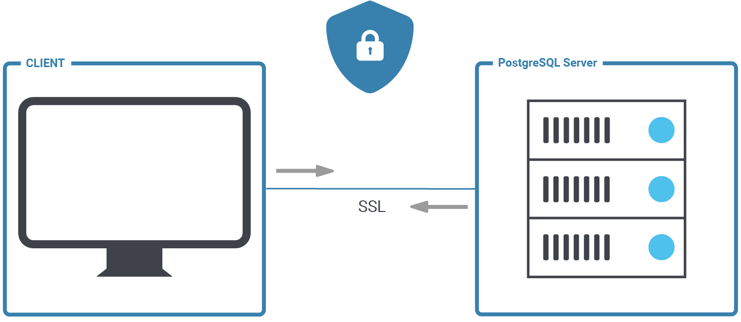
PostgreSQL is a secure database and we want to keep it that way. It makes sense, then, to consider SSL to encrypt the connection between client and server. This posting will help you to set up SSL authentication for PostgreSQL properly, and hopefully also to understand some background information to make your database more secure.
At the end of this post, you should be able to configure PostgreSQL and handle secure client server connections in the easiest way possible.
The first thing we have to do to set up OpenSSL is to change postgresql.conf. There are a couple of parameters which are related to encryption:
|
1 2 3 4 5 6 7 8 9 10 11 12 13 |
ssl = on #ssl_ca_file = '' #ssl_cert_file = 'server.crt' #ssl_crl_file = '' #ssl_key_file = 'server.key' #ssl_ciphers = 'HIGH:MEDIUM:+3DES:!aNULL' # allowed SSL ciphers #ssl_prefer_server_ciphers = on #ssl_ecdh_curve = 'prime256v1' #ssl_min_protocol_version = 'TLSv1.2' #ssl_max_protocol_version = '' #ssl_dh_params_file = '' #ssl_passphrase_command = '' #ssl_passphrase_command_supports_reload = off |
Once ssl = on, the server will negotiate SSL connections in case they are possible. The remaining parameters define the location of key files and the strength of the ciphers. Please note that turning SSL on does not require a database restart. The variable can be set with a plain reload. However, you will still need a restart, otherwise PostgreSQL will not accept SSL connections. This is an important point which frequently causes problems for users:
|
1 2 3 4 5 6 7 8 9 10 11 |
postgres=# SELECT pg_reload_conf(); pg_reload_conf ---------------- t (1 row) postgres=# SHOW ssl; ssl ----- on (1 row) |
The SHOW command is an easy way to make sure that the setting has indeed been changed. Technically, pg_reload_conf() is not needed at this stage. It is necessary to restart later anyway. We just reloaded to show the effect on the variable.
In the next step, we have to adjust pg_hba.conf to ensure that PostgreSQL will handle our connections in a secure way:
|
1 2 3 4 5 6 7 |
# TYPE DATABASE USER ADDRESS METHOD # 'local' is for Unix domain socket connections only local all all peer host all all 127.0.0.1/32 scram-sha-256 host all all ::1/128 scram-sha-256 hostssl all all 10.0.3.0/24 scram-sha-256 |
Then restart the database instance to make sure SSL is enabled.
In order to keep things simple, we will simply create self-signed certificates here. However, it is of course also possible with other certificates are. Here is how it works:
|
1 2 3 4 5 6 7 8 9 |
[postgres@node1 data]$ openssl req -new -x509 -days 365 -nodes -text -out server.crt -keyout server.key -subj '/CN=cybertec-postgresql.com' Generating a RSA private key .......+++++ ....................................................+++++ writing new private key to 'server.key' ----- |
This certificate will be valid for 365 days.
Next we have to set permissions to ensure the certificate can be used. If those permissions are too relaxed, the server will not accept the certificate:
|
1 |
[postgres@node1 data]$ chmod og-rwx server.key |
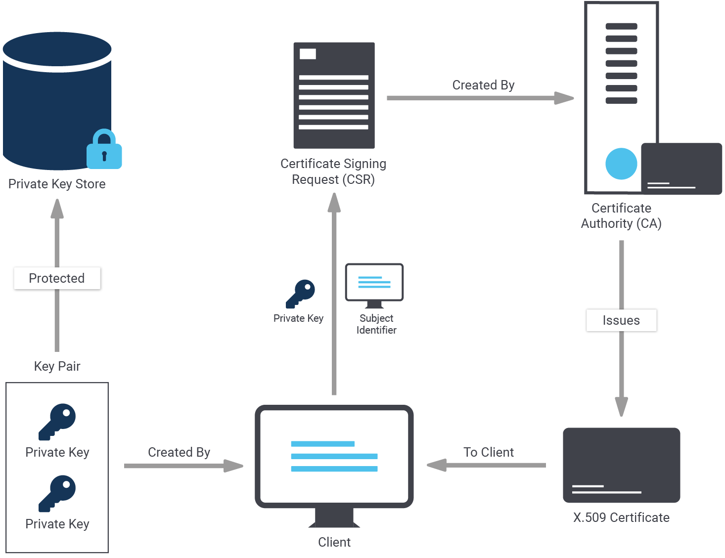
Self-signed certificates are nice. However, to create a server certificate whose identity and origin can be validated by clients, first create a certificate signing request and a public/private key file:
|
1 2 3 4 5 6 7 8 9 |
[postgres@node1 data]$ openssl req -new -nodes -text -out root.csr -keyout root.key -subj '/CN=cybertec-postgresql.com' Generating a RSA private key .................................+++++ ....................+++++ writing new private key to 'root.key' ----- |
Again, we have to make sure that those permissions are exactly the way they should be:
|
1 |
[postgres@node1 data]$ chmod og-rwx root.key |
To do that with OpenSSL, we first have to find out where openssl.cnf can be found. We have seen that it is not always in the same place - so make sure you are using the right path:
|
1 2 3 |
[postgres@node1 data]$ find / -name openssl.cnf 2> /dev/null /etc/pki/tls/openssl.cnf |
We use this path when we sign the request:
|
1 2 3 4 5 6 7 8 9 |
[postgres@node1 data]$ openssl x509 -req -in root.csr -text -days 3650 -extfile /etc/pki/tls/openssl.cnf -extensions v3_ca -signkey root.key -out root.crt Signature ok subject=CN = cybertec-postgresql.com Getting Private key |
Let’s create the certificate with the new root authority:
|
1 2 3 4 5 6 7 8 9 10 11 12 13 14 15 16 |
[postgres@node1 data]$ openssl req -new -nodes -text -out server.csr -keyout server.key -subj '/CN=cybertec-postgresql.com' Generating a RSA private key .....................+++++ ...........................+++++ writing new private key to 'server.key' [postgres@node1 data]$ chmod og-rwx server.key [postgres@node1 data]$ openssl x509 -req -in server.csr -text -days 365 -CA root.crt -CAkey root.key -CAcreateserial -out server.crt Signature ok subject=CN = cybertec-postgresql.com Getting CA Private Key |
server.crt and server.key should be stored on the server in your data directory as configured on postgresql.conf.
But there's more: root.crt should be stored on the client, so the client can verify that the server's certificate was signed by the certification authority. root.key should be stored offline for use in creating future certificates.
The following files are needed:
| File name | Purpose of the file | Remarks |
| ssl_cert_file ($PGDATA/server.crt) | server certificate | sent to client to indicate server's identity |
| ssl_key_file ($PGDATA/server.key) | server private key | proves server certificate was sent by the owner; does not indicate certificate owner is trustworthy |
| ssl_ca_file | trusted certificate authorities | checks that client certificate is signed by a trusted certificate authority |
| ssl_crl_file | certificates revoked by certificate authorities | client certificate must not be on this list |
Now that all the certificates are in place it is time to restart the servers:
|
1 |
[root@node1 ~]# systemctl restart postgresql-13 |
Without a restart, the connection would fail with an error message (“psql: error: FATAL: no pg_hba.conf entry for host "10.0.3.200", user "postgres", database "test", SSL off”).
However, after the restart, the process should work as expected:
|
1 2 3 4 5 6 7 8 |
[root@node1 ~]# su - postgres [postgres@node1 ~]$ psql test -h 10.0.3.200 Password for user postgres: psql (13.2) SSL connection (protocol: TLSv1.3, cipher: TLS_AES_256_GCM_SHA384, bits: 256, compression: off) Type 'help' for help. test=# |
psql indicates that the connection is encrypted. To figure out if the connection is indeed encrypted, we need to check the content of pg_stat_ssl:
|
1 2 3 4 5 6 7 8 9 10 11 12 13 14 |
postgres=# d pg_stat_ssl View 'pg_catalog.pg_stat_ssl' Column | Type | Collation | Nullable | Default ----------------+---------+-----------+----------+--------- pid | integer | | | ssl | boolean | | | version | text | | | cipher | text | | | bits | integer | | | compression | boolean | | | client_dn | text | | | client_serial | numeric | | | issuer_dn | text | | | |
Let us query the system view and see what it contains:
|
1 2 3 4 5 6 7 8 9 10 11 12 13 |
test=# x Expanded display is on. test=# SELECT * FROM pg_stat_ssl; -[ RECORD 1 ]-+----------------------- pid | 16378 ssl | t version | TLSv1.3 cipher | TLS_AES_256_GCM_SHA384 bits | 256 compression | f client_dn | client_serial | issuer_dn | |
The connection has been successfully encrypted. If “ssl = true”, then we have succeeded.
Two SSL setups are not necessarily identical. There are various levels which allow you to control the desired level of security and protection. The following table outlines those SSL modes as supported by PostgreSQL:
sslmode | Eavesdropping protection | MITM (= man in the middle) protection | Statement |
| disable | No | No | No SSL, no encryption and thus no overhead. |
| allow | Maybe | No | The client attempts an unencrypted connection, but uses an encrypted connection if the server insists. |
| prefer | Maybe | No | The reverse of the “allow” mode: the client attempts an encrypted connection, but uses an unencrypted connection if the server insists. |
| require | Yes | No | Data should be encrypted and the overhead of doing so is accepted. The network is trusted and will send me to the desired server. |
| verify-ca | Yes | Depends on CA policy | Data must be encrypted. Systems must be doubly sure that the connection to the right server is established. |
| verify-full | Yes | Yes | Strongest protection possible. Full encryption and full validation of the desired target server. |
The overhead really depends on the mode you are using. First let’s take a look at the general mechanism:
The main question now is: How does one specify the mode to be used? The answer is: It has to be hidden as part of the connect string as shown in the next example:
|
1 2 3 |
[postgres@node1 data]$ psql 'dbname=test host=10.0.3.200 user=postgres password=1234 sslmode=verify-ca' psql: error: root certificate file '/var/lib/pgsql/.postgresql/root.crt' does not exist Either provide the file or change sslmode to disable server certificate verification. |
In this case, verify-ca does not work because to do that the root.* files have to be copied to the client, and the certificates have to be ones which allow for proper validation of the target server.
So far, you have learned how to encrypt the connection between client and server. However, sometimes it is necessary to encrypt the entire server, including storage. PostgreSQL TDE does exactly that:
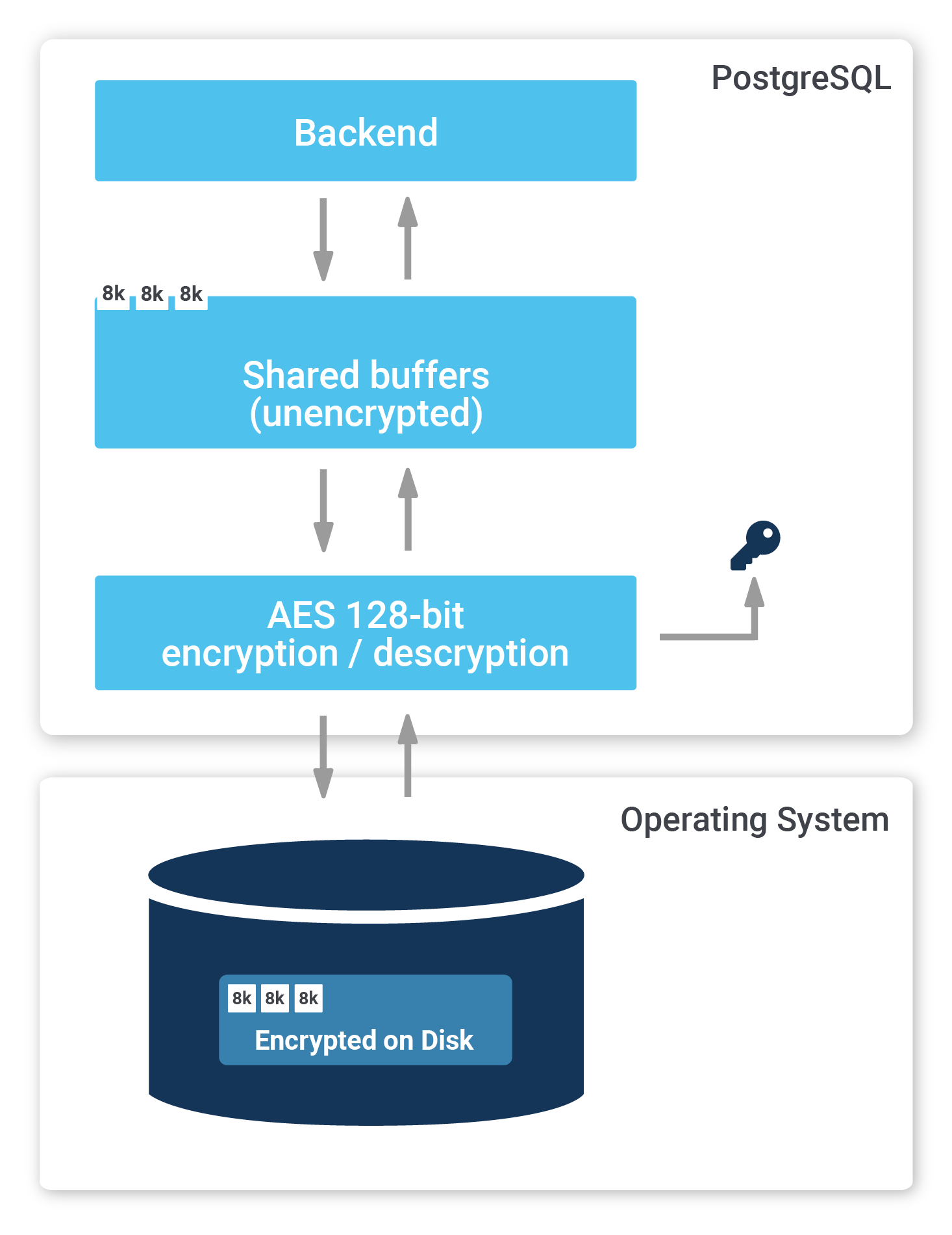
To find out more, check out our website about PostgreSQL TDE. We offer a fully encrypted stack to help you achieve maximum security. PostgreSQL TDE is available for free (Open Source).
More recent information about encryption keys: Manage Encryption Keys with PostgreSQL TDE
Materialized views are an important feature in most databases, including PostgreSQL. They can help to speed up large calculations, or at least to cache them.
If you want to make sure that your materialized views are up-to-date, and if you want to read more about PostgreSQL right now, check out our blog about pg_timetable, which shows you how to schedule jobs in PostgreSQL. Why is pg_timetable so useful? Our scheduler makes sure that identical jobs cannot overlap, but simply don’t execute again in case the same job is already running. In the case of long jobs, using a scheduler is super important - especially if you want to use materialized views.
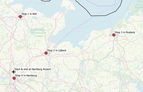
Last time, we experimented with lesser known PostGIS functions to extract areas of interest for sales. Now, let’s extend our example regarding catchment areas by optimizing trips within the area of interest we generated in our previous example, which is around Hamburg. Let’s ask the following question:
which order should we visit our major cities in so that we can optimize our trip’s costs?
This optimization problem is commonly known as the Traveling Salesman Problem (or TSP).
Apart from PostGIS, pgRouting will be used to tackle this challenge within PostgreSQL only. pgRouting is served as a PostgreSQL extension, which adds a lot of geospatial routing functionality on top of PostGIS.
I recommend you check out its online documentation, located at https://pgrouting.org/, to get an overview.
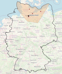 | 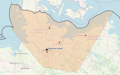 |
Figure 1 Area of interest around Hamburg / Figure 2 Area of interest around Hamburg, Zoom
This article is organized as follows:
We will re-use osm files and datasets processed in my last blogpost, so first, please play through the blogpost sections involved. Subsequently, an intermediate table “tspPoints” must be created, which contains major cities and airports covered by our preferred area around Hamburg only (see the annex for ddl).
To solve TSP by utilizing our pgRouting functionality, we must generate a graph out of osm data. Different tools like osm2pgrouting or osm2po exist, which generate a routable graph from plain osm data. Due to limited memory resources on my development machine, I decided to give osm2po a try.
So then - let’s start. After downloading the latest osm2po release from https://osm2po.de/releases/,
we need to adapt its configuration, in order to generate the desired graph as an sql file.
Please uncomment the following line in osm2po.config to accomplish this task.
postp.0.class = de.cm.osm2po.plugins.postp.PgRoutingWriter
Now we’re ready to generate our graph by executing
|
1 2 |
java -Xmx8g -jar osm2po-core-x.x.x-signed.jar workDir=/data/de-graph prefix=de tileSize=x /data/germany-latest.osm.pbf |
The outputted sql file can easily be imported to PostGIS by calling
|
1 |
psql -U username -d dbname -q -f /data/de-graph/de_2po_4pgr.sql |
the resulting graph table contains geometries for edges only (see annex for ddl). To generate source and target nodes too, let’s utilize pgr_createverticestable as follows:
|
1 2 |
select pgr_createverticestable('de_2po_4pgr', 'geom_way', 'source', 'target'); |
Slowly, we’re getting closer ????. Figure 3 to 5 represent our stacked layer setup on top of OpenStreetMap, which is based upon the following tables:
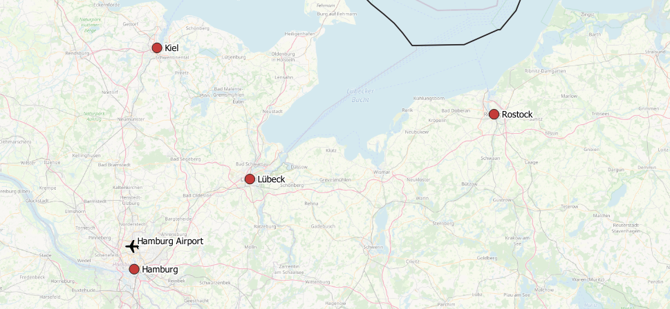 Figure 3 Intermediate trip stops | |
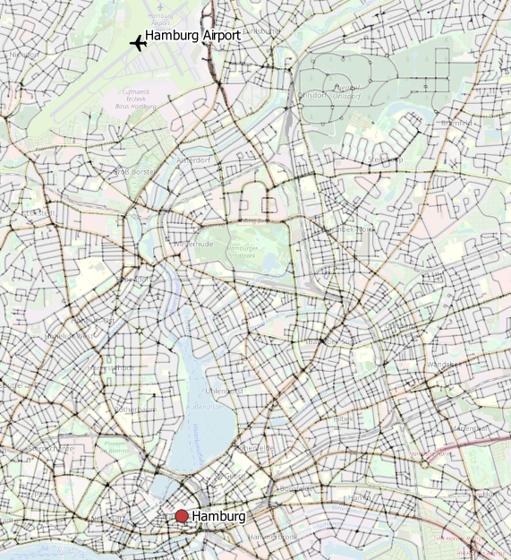 Figure 4 Edges around Hamburg |  Figure 5 Edges + nodes around Hamburg |
Now let’s ask pgRouting to solve our traveling salesmen problem by querying
|
1 2 3 4 5 6 7 8 9 10 11 12 13 14 |
SELECT seq,node, cost, agg_cost FROM pgr_TSP( $$ SELECT * FROM pgr_dijkstraCostMatrix( 'SELECT id, source, target, cost, reverse_cost FROM de_2po_4pgr', (with nearestVertices as( SELECT a.id from tsppoints, lateral ( select id,the_geom from osmtile_germany.de_2po_4pgr_vertices_pgr order by osmtile_germany.de_2po_4pgr_vertices_pgr.the_geom <-> osmtile_germany.tsppoints.geom limit 1 ) a) select array_agg(id) from nearestVertices), directed := false) $$, start_id := 591341); |
This command results in the optimal order of intermediate stops (edges next to our cities) forming our trip. It’s worth pointing out that the optimal route (order) depends on the cost-matrix’s respective cost-function, which was defined to calculate the edge’s weights. In our case, the cost function is prescribed by osm2po and expressed as length/kmh.
To export the sequence of city names to pass through, the nodes returned by pgr_TSP must be joined back to tspPoints. Please consult the annex for this particular query extension. From figure 6 we now realize that the optimal route goes from Hamburg Airport to Kiel, Lübeck, Rostock and Hamburg before bringing us back to our airport.
This time, we took a quick look at pgRouting to solve a basic traveling salesman problem within PostGIS. Feel free to experiment with further cost functions and to move on to calculating detailed routes between cities by utilizing further pgRouting functions.
|
1 2 3 4 5 6 7 8 9 10 11 12 13 14 15 16 17 18 19 20 21 22 23 24 25 26 27 28 29 30 31 32 33 |
create table if not exists osmtile_germany.de_2po_4pgr ( id integer not null constraint pkey_de_2po_4pgr primary key, osm_id bigint, osm_name varchar, osm_meta varchar, osm_source_id bigint, osm_target_id bigint, clazz integer, flags integer, source integer, target integer, km double precision, kmh integer, cost double precision, reverse_cost double precision, x1 double precision, y1 double precision, x2 double precision, y2 double precision, geom_way geometry(LineString,4326) ); create index if not exists idx_de_2po_4pgr_source on osmtile_germany.de_2po_4pgr (source); create index if not exists idx_de_2po_4pgr_target on osmtile_germany.de_2po_4pgr (target); create index if not exists idx_de_2po_geom on osmtile_germany.de_2po_4pgr using gist (geom_way); |
|
1 2 3 4 5 6 7 8 |
create table osmtile_germany.tspPoints ( id serial primary key, name text, geom geometry(Point, 4326) ); create index idx_tspPoints on osmtile_germany.tspPoints using gist (geom); |
|
1 2 3 4 5 6 7 8 9 10 11 12 13 14 15 16 17 18 19 20 21 22 23 24 25 26 27 28 29 30 31 32 33 34 35 36 37 38 39 40 |
SELECT seq, node, a.name, a.geom FROM pgr_TSP( $ SELECT * FROM pgr_dijkstraCostMatrix( 'SELECT id, source, target, cost, reverse_cost FROM de_2po_4pgr', ( with nearestVertices as( SELECT a.id from tsppoints, lateral ( select id, the_geom from osmtile_germany.de_2po_4pgr_vertices_pgr order by osmtile_germany.de_2po_4pgr_vertices_pgr.the_geom <-> osmtile_germany.tsppoints.geom limit 1 ) a ) select array_agg(id) from nearestVertices ), directed := false )$, start_id := 591341 ), de_2po_4pgr_vertices_pgr, lateral ( select name, geom from osmtile_germany.tsppoints order by osmtile_germany.tsppoints.geom <-> the_geom limit 1 ) a where node = id |
by Kaarel Moppel
The big question we hear quite often is, “Can and should we run production Postgres workloads in Docker? Does it work?” The answer in short: yes, it will work... if you really want it to... or if it’s all only fun and play, i.e. for throwaway stuff like testing.
Containers, commonly also just called Docker, have definitely been a thing for quite a few years now. (There are other popular container runtimes out there, and it’s not a proprietary technology per se, but let’s just say Docker to save on typing.) More and more people are “jumping on the container-ship” and want to try out Docker, or have already given this technology a go. However, containers were originally designed more as a vehicle for code; they were initially intended to provide a worry-free “batteries included” deployment experience. The idea is that it “just works” anywhere and is basically immutable. That way, quality can easily be tested and guaranteed across the board.
Those are all perfectly desirable properties indeed for developers...but what if you’re in the business of data and database management? Databases, as we know, are not really immutable - they maintain a state, so that code can stay relatively “dumb” and doesn’t have to “worry” about state. Statelessness enables rapid feature development and deployment, and even push-button scaling - just add more containers!

If your sensors are halfway functional, you might have picked up on some concerned tones in that last statement, meaning there are some “buts” - as usual. So why not fully embrace this great modern technology and go all in? Especially since I already said it definitely works.
The reason is that there are some aspects you should at least take into account to avoid cold sweats and swearing later on. To summarise: you’ll benefit greatly for your production-grade use cases only if you’re ready to do the following:
a) live fully on a container framework like Kubernetes / OpenShift
b) depend on some additional 3rd party software projects not directly affiliated with the PostgreSQL Global Development Group
c) or maintain either your own Docker images, including some commonly needed extensions, or some scripts to perform common operational tasks like upgrading between major versions.
To reiterate - yes, containers are mostly a great technology, and this type of stuff is interesting and probably would look cool on your CV...but: the origins of container technologies do not stem from persistent use cases. Also, the PostgreSQL project does not really do much for you here besides giving you a quick and convenient way to launch a standard PostgreSQL instance on version X.
Not to sound too discouraging - there is definitely at least one perfectly valid use case out there for Docker / containers: it’s perfect for all kinds of testing, especially for integration and smoke testing!
Since we basically implement containers as super light-weight “mini VMs”, you can start and discard them in seconds! That, however, assumes you have already downloaded the image. If not, then the first launch will take a minute or two, depending on how good your internet connection is 🙂
As a matter of fact, I personally usually have all the recent (9.0+) versions of Postgres constantly running on my workstation in the background, via Docker! I don’t of course use all those versions too frequently - however, since they don’t ask for too much attention, and don’t use up too many resources if “idling”, they don’t bother me. Also, they’re always there for me when I need to test out some Postgres statistic fetching queries for our Postgres monitoring tool called pgwatch2. The only annoying thing that could pester you a bit is - if you happen to also run Postgres on the host machine, and want to take a look at a process listing to figure out what it’s doing, (e.g. ps -efH | grep postgres) the “in container” processes show up and somewhat “litter” the picture.
OK, so I want to benefit from those light-weight pre-built “all-inclusive” database images that everyone is talking about and launch one - how do I get started? Which images should I use?
As always, you can’t go wrong with the official stuff - and luckily, the PostgreSQL project provides all modern major versions (up to v8.4 by the way, released in 2009!) via the official Docker Hub. You also need to know some “Docker foo”. For a simple test run, you usually want something similar to what you can see in the code below.
NB! As a first step, you need to install the Docker runtime / engine (if it is not already installed). I’ll not be covering that, as it should be a simple process of following the official documentation line by line.
Also note: when launching images, we always need to explicitly expose or “remap” the default Postgres port to a free port of our preference. Ports are the “service interface” for Docker images, over which all communication normally happens. So we actually don’t need to care about how the service is internally implemented!
|
1 2 3 4 5 6 7 8 9 |
# Note that the first run could take a few minutes due to the image being downloaded… docker run -d --name pg13 -p 5432:5432 -e POSTGRES_HOST_AUTH_METHOD=trust postgres:13 # Connect to the container that’s been started and display the exact server version psql -U postgres -h localhost -p 5432 -c 'show server_version' postgres server_version ──────────────────────────────── 13.1 (Debian 13.1-1.pgdg100+1) (1 row) |
Note that you don’t have to actually use “trust” authentication, but can also set a password for the default “postgres” superuser via the POSTGRES_PASSWORD env variable.
Once you’ve had enough of Slonik’s services for the time being, just throw away the container and all the stored tables / files etc with the following code:
|
1 2 3 4 |
# Let’s stop the container / instance docker stop pg13 # And let’s also throw away any data generated and stored by our instance docker rm pg13 |
Couldn’t be any simpler!
NB! Note that I could also explicitly mark the launched container as “temporary” with the ‘--rm’ flag when launching the container, so that any data remains would automatically be destroyed upon stopping.
Now that we have seen how basic container usage works, complete Docker beginners might get curious here - how does it actually function? What is actually running down there inside the container box?
First, we should probably clear up the two concepts that people often initially mix up:
Let’s make sense of this visually:
|
1 2 3 4 5 6 7 8 9 10 11 12 13 14 15 16 17 18 19 |
# Let’s take a look at available Postgres images on my workstation # that can be used to start a database service (container) in the snappiest way possible docker images | grep ^postgres | sort -k2 -n postgres 9.0 cd2eca8588fb 5 years ago 267MB postgres 9.1 3a9dca7b3f69 4 years ago 261MB postgres 9.2 18cdbca56093 3 years ago 261MB postgres 9.4 ed5a45034282 12 months ago 251MB postgres 9.5 693ab34b0689 2 months ago 197MB postgres 9.6 ebb1698de735 6 months ago 200MB postgres 10 3cfd168e7b61 3 months ago 200MB postgres 11.5 5f1485c70c9a 16 months ago 293MB postgres 11 e07f0c129d9a 3 months ago 282MB postgres 12 386fd8c60839 2 months ago 314MB postgres 13 407cece1abff 14 hours ago 314MB # List all running containers docker ps CONTAINER ID IMAGE COMMAND CREATED STATUS PORTS NAMES 042edf790362 postgres:13 'docker-entrypoint.s…' 11 hours ago Up 11 hours 0.0.0.0:5432->5432/tcp pg13 |
Other common tasks when working with Docker might be:
|
1 2 3 4 |
# Get all log entries since initial launch of the instance docker logs pg13 # “Tail” the logs limiting the initial output to last 10 minutes docker logs --since '10m' --follow pg13 |
Note that by default, all Docker containers can speak to each other, since they get assigned to the default subnet of 172.17.0.0/16. If you don’t like that, you can also create custom networks to cordon off some containers, whereby then they can also access each other using the container name!
|
1 2 3 4 5 6 |
# Simple ‘exec’ into container approach docker exec -it pg13 hostname -I 172.17.0.2 # A more sophisticated way via the “docker inspect” command docker inspect -f '{{range.NetworkSettings.Networks}}{{.IPAddress}}{{end}}' pg13 |
Note that this should be a rather rare occasion, and is usually only necessary for some troubleshooting purposes. You should try not to install new programs and change the files directly, as this kind of defeats the concept of immutability. Luckily, in the case of official Postgres images you can easily do that, since it runs under “root” and the Debian repositories are also still connected - which a lot of images remove, in order to prevent all sorts of maintenance nightmares.
Here is an example of how to install a 3rd party extension. By default, we only get the “contrib extensions” that are part of the official Postgres project.
|
1 2 3 4 5 6 7 8 |
docker exec -it pg13 /bin/bash # Now we’re inside the container! # Refresh the available packages listing apt update # Let’s install the extension that provides some Oracle compatibility functions... apt install postgresql-13-orafce # Let’s exit the container (can also be done with CTRL+D) exit |
Quite often when doing some application testing, you want to measure how much time the queries really take - i.e. measure things from the DB engine side via the indispensable “pg_stat_statements” extension. You can do it relatively easily, without going “into” the container! Starting from Postgres version 9.5, to be exact...
|
1 2 3 4 5 6 7 8 9 10 11 |
# Connect with our “Dockerized” Postgres instance psql -h localhost -U postgres postgres=# ALTER SYSTEM SET shared_preload_libraries TO pg_stat_statements; ALTER SYSTEM postgres=# ALTER SYSTEM SET track_io_timing TO on; ALTER SYSTEM # Exit psql via typing “exit” or pressing CTRL+D # and restart the container docker restart pg13 |
As stated in the Docker documentation: “Ideally, very little data is written to a container’s writable layer, and you use Docker volumes to write data.”
The thing about containers’ data layer is that it’s not really meant to be changed! Remember, containers should be kind of immutable. The way it works internally is via “copy-on-write”. Then, there’s a bunch of different storage drivers used over different versions of historical Docker runtime versions. Also, there are some differences which spring from different host OS versions. It can get quite complex, and most importantly, slow on the disk access level via the “virtualized” file access layer. It’s best to listen to what the documentation says, and set up volumes for your data to begin with.
They’re directly connected and persistent OS folders where Docker tries to stay out of the way as much as possible. That way, you don’t actually lose out on file system performance and features. The latter is not really guaranteed, though - and can be platform-dependent. Things might look a bit hairy, especially on Windows (as usual), where one nice issue comes to mind. The most important keyword here might be “persistent” - meaning volumes don’t disappear, even when a container is deleted! So they can also be used to “migrate” from one version of the software to another.
How should you use volumes, in practice? There are two ways to use volumes: the implicit and the explicit. The “fine print” by the way, is available here.
Also, note that we actually need to know beforehand what paths should be directly accessed, i.e. “volumized”! How can you find out such paths? Well, you could start from the Docker Hub “postgres” page, or locate the instruction files (the Dockerfile) that are used to build the Postgres images and search for the “VOLUME” keyword. The latter can be found for Postgres here.
|
1 2 3 4 5 6 7 8 9 10 11 12 13 14 15 |
# Implicit volumes: Docker will automatically create the left side folder if it is not already there docker run -d --name pg13 -p5432:5432 -e POSTGRES_HOST_AUTH_METHOD=trust -v /mydatamount/pg-persistent-data:/var/lib/postgresql/data postgres:13 # Explicit volumes: need to be pre-initialized via Docker docker volume create pg13-data docker run -d --name pg13 -p5432:5432 -e POSTGRES_HOST_AUTH_METHOD=trust -v pg13-data:/var/lib/postgresql/data postgres:13 # Let’s inspect where our persistent data actually “lives” docker volume inspect pg13-data # To drop the volume later if the container is not needed anymore use the following command docker volume rm pg13-data |
To tie up the knots on this posting - if you like containers in general, and also need to run some PostgreSQL services - go ahead! Containers can be made to work pretty well, and for bigger organizations running hundreds of PostgreSQL services, it can actually make life a lot easier and more standardized once everything has been automated. Most of the time, the containers won’t bite you.
But at the same time, you had better be aware of the pitfalls:
Don’t want to sound like a luddite again, but before going “all in” on containers you should acknowledge two things. One, that there are major benefits to production-level database containers only if you’re using some container automation platform like Kubernetes. Two, the benefits will come only if you are willing to make yourself somewhat dependent on some 3rd party software vendors. 3rd party vendors are not out to simplify the life of smaller shops, but rather cater to bigger “K8s for the win” organizations. Often, they encode that way of thinking into the frameworks, which might not align well with your way of doing things.
Also, not all aspects of the typical database lifecycle are well covered. My recommendation is: if it currently works for you “as is”, and you’re not 100% migrating to some container-orchestration framework for all other parts of your software stack, be aware that you’re only winning in the ease of the initial deployment and typically also in automatic high-availability (which is great of course!) - but not necessarily in all aspects of the whole lifecycle (fast major version upgrades, backups the way you like them, access control, etc).
On the other hand - if you feel comfortable with some container framework like Kubernetes and/or can foresee that you’ll be running oodles of database instances - give it a go! -- after you research possible problem points, of course.
On the positive side - since I am in communication with a pretty wide crowd of DBA’s, I can say that many bigger organizations do not want to look back at the traditional way of running databases after learning to trust containers.
Anyway, it went a bit long - thanks for reading, and please do let me know in the comments section if you have some thoughts on the topic!
GitHub Actions (GHA) are altogether a piece of excellent machinery for continuous integration or other automated tasks on your repo. I started to use them from the release day on as a replacement for CircleCI. Not that I think CircleCI is a bad product; I love to have everything in one place if possible. However, using a young product is a challenge. Even now, there is no easy way to debug actions.
I came up with many solutions: Docker-based actions, actions downloading binaries, etc. But this post will cover using the latest GitHub Actions Virtual Environments, which have PostgreSQL installed by default. Handy, huh? 🙂
Here is the table listing all available GitHub Actions Virtual Environments for a moment:
| Environment | YAML Label | Included Software |
|---|---|---|
| Ubuntu 20.04 | ubuntu-20.04 |
ubuntu-20.04 |
| Ubuntu 18.04 | ubuntu-latest or ubuntu-18.04 |
ubuntu-18.04 |
| Ubuntu 16.04 | ubuntu-16.04 |
ubuntu-16.04 |
| macOS 11.0 | macos-11.0 |
macOS-11.0 |
| macOS 10.15 | macos-latest or macos-10.15 |
macOS-10.15 |
| Windows Server 2019 | windows-latest or windows-2019 |
windows-2019 |
| Windows Server 2016 | windows-2016 |
windows-2016 |
In this post, I will use three of them: windows-latest, ubuntu-latest, and macos-latest. However, you may use any of the environments available. These actions were first written for pg_timetable testing, but now they are used as a template for all Cybertec PostgreSQL-related actions.
Each of the actions below will:
scheduler;timetable.Of course, you may want to add more steps in real life, e.g., import test data, checkout, build, test, gather coverage, release, etc.
|
1 2 3 4 5 6 7 8 9 10 11 12 13 14 15 16 |
setup-postgresql-ubuntu: if: true # false to skip job during debug name: Setup PostgreSQL on Ubuntu runs-on: ubuntu-latest steps: - name: Start PostgreSQL on Ubuntu run: | sudo systemctl start postgresql.service pg_isready - name: Create scheduler user run: | sudo -u postgres psql --command='CREATE USER scheduler PASSWORD 'somestrong'' --command='du' - name: Create timetable database run: | sudo -u postgres createdb --owner=scheduler timetable PGPASSWORD=somestrong psql --username=scheduler --host=localhost --list timetable |
Nothing unusual here for Ubuntu users. We use systemctl to start PostgreSQL and the pg_isready utility to check if the server is running.
To create a scheduler user, we use a psql client in non-interactive mode. We send two commands to it:
CREATE USER ...;du — list users.First, we create the user. Second, we output the list of users for control.
💡 To remember psql commands, try to decode them. For example,
dt- describe tables,du- describe users, etc.
To create a timetable database, we use the createdb utility. Pay attention to the fact that sudo -u postgres allows us to not specify connection credentials, because a system user is allowed to connect locally without any restrictions. Then, just like in the previous step, list the databases with psql for control.
|
1 2 3 4 5 6 7 8 9 10 11 12 13 14 15 16 17 18 19 20 21 22 23 24 25 26 27 28 29 30 |
setup-postgresql-macos: if: true # false to skip job during debug name: Setup PostgreSQL on MacOS runs-on: macos-latest steps: - name: Start PostgreSQL on MacOS run: | brew services start postgresql echo 'Check PostgreSQL service is running' i=10 COMMAND='pg_isready' while [ $i -gt 0 ]; do echo 'Check PostgreSQL service status' eval $COMMAND && break ((i--)) if [ $i == 0 ]; then echo 'PostgreSQL service not ready, all attempts exhausted' exit 1 fi echo 'PostgreSQL service not ready, wait 10 more sec, attempts left: $i' sleep 10 done # Homebrew creates an account with the same name as the installing user, but no password - name: Create scheduler user run: | psql --command='CREATE USER scheduler PASSWORD 'somestrong'' --command='du' postgres - name: Create timetable database run: | createdb --owner=scheduler timetable PGPASSWORD=somestrong psql --username=scheduler --host=localhost --list timetable |
There are not so many differences from Ubuntu for MacOS:
brew services to start the server;pg_isready procedure is more complicated.As you probably noticed, we may skip sudo -u postgres prefixes since the current user has all the rights needed in this environment.
|
1 2 3 4 5 6 7 8 9 10 11 12 13 14 15 16 17 18 |
setup-postgresql-windows: if: true # false to skip job during debug name: Setup PostgreSQL on Windows runs-on: windows-latest steps: - name: Start PostgreSQL on Windows run: | $pgService = Get-Service -Name postgresql* Set-Service -InputObject $pgService -Status running -StartupType automatic Start-Process -FilePath '$env:PGBINpg_isready' -Wait -PassThru - name: Create scheduler user on Windows run: | & $env:PGBINpsql --command='CREATE USER scheduler PASSWORD 'somestrong'' --command='du' - name: Create timetable database run: | & $env:PGBINcreatedb --owner=scheduler timetable $env:PGPASSWORD = 'somestrong' & $env:PGBINpsql --username=scheduler --host=localhost --list timetable |
With Windows, everything is different, but not as scary as haters usually paint it to be:
pwsh) by default;I think the code is straightforward. The only thing I want to highlight is the ampersand sign (& aka call operator) before some commands.
The call operator (&) allows you to execute a command, script, or function. Since the PostgreSQL utilities psql and createdb are not in the PATH, we need to specify the full path to them. We use the environmental variable PGBIN for that. But after the concatenation operation, we have a regular string. Therefore, a call operator allows us to execute a resulting command.
💡 PowerShell (
pwsh) is available for all environments in GitHub Actions including Ubuntu and macOS. That's a pretty powerful shell, I must say! Try to give it a chance and you will be surprised.
There are also other ways to run PostgreSQL within GitHub Actions. Let me know if you are interested in this topic, and I will write again with even more examples.
In conclusion, I wish you all the best! ♥️
Please, stay safe! So we can meet in person at one of the conferences, meetups, or training sessions.
PostgreSQL commit ee28cacf61 has added new options for the target_session_attrs connection parameter. This article explores how the new options can be used to simplify high availability and horizontal scaling solutions.
target_session_attrs?The PostgreSQL client shared library libpq has support for connection strings to more than one database server:
|
1 |
psql 'host=server1.my.org,server2.my.org port=5432,5432 dbname=mydb user=myself' |
In the URL connection string format, that would look like
|
1 |
psql 'postgresql://myself@server1.my.org:5432,server2.my.org:5432/mydb' |
Then the client will first try to connect to server1.my.org, and if it cannot reach that server, it will try to connect to server2.my.org.
This is useful in combination with high-availability solutions, because it allows the client to fail over to a secondary server without the need for additional load balancing software. However, there is one shortcoming: if we don't know which of the servers is the currently active primary server, we might accidentally end up connecting to a standby server. This is usually not what you want, because you cannot run data modifying statements there.
To make up for this, you can specify the additional parameter “target_session_attrs”, which determines when a server is acceptable. If you specify
|
1 |
target_session_attrs=read-write |
the PostgreSQL client will not accept a connection to a server where it cannot modify data. This allows you to connect to the streaming replication primary, regardless of the order of the servers in the connection string.
target_session_attrs in v14PostgreSQL v14 introduces these new options:
read-only: only connect to a server that does not allow data modifications. This is the converse of read-write.primary: only connect to a database that is not a streaming replication standby.standby: only connect to a streaming replication standby.prefer-standby: connect to a standby server if there is one. Only if there is no standby server on the list, accept a connection to a server that is not in recovery mode.You are probably confused by the distinction between “read-only” and “standby” or between “read-write” and “primary”.
The difference is subtle: if the parameter “default_transaction_read_only” is set to “on”, a server can be read-only even if it is not a streaming replication standby server.
target_session_attrs?Since this functionality is part of the client C library libpq, all clients that link with that library automatically support this connection parameter. This includes the Python library psycopg2, drivers for Go, Rust and most other programming languages.
Notable exceptions to this are the PostgreSQL JDBC driver and the .NET provider Npgsql, which do not link with libpq. However, the JDBC driver already has support for this functionality with the “targetServerType” connection parameter, which you can set to “primary”, “secondary” and “preferSecondary” to achieve the same behavior. Npgsql does not offer this functionality.
target_session_attrs for high availabilityThe application is obvious: you always want to connect to the primary server. While target_session_attrs=read-write served the purpose fairly well, you should switch to using target_session_attrs=primary. This will do the right thing even in the unlikely case that somebody set default_transaction_read_only on the primary server.
target_session_attrs for horizontal scalingYou can use PostgreSQL streaming replication for horizontal scaling by directing read requests to standby servers. There are some limitations to this approach:
Other than that, you can use target_session_attrs to implement scaling without the need for additional load balancing software:
target_session_attrs=read-write.target_session_attrs=prefer-standby. If you have more than one standby server, you could also use standby — then your application will fail rather than directing read requests to the primary server.The new settings for target_session_attrs allow a more reliable high-availability setup and some degree of horizontal scaling without the need for additional software. This can simplify your architecture, thus making it more reliable.
To make it easier for our readers to install PostgreSQL on Ubuntu, we have compiled a quick guide to getting started. Don’t worry, it’s not too hard. You will learn:
Note that this is an introduction. If you are looking to create a PostgreSQL High-Availability cluster, we recommend checking out some of our other content.
For this demonstration I have created a virtual machine using VirtualBox on my local machine. We use Ubuntu 20.10 in this tutorial.
Installing Ubuntu on VirtualBox is easy. Simply download the Ubuntu ISO file from the website and create a virtual machine:
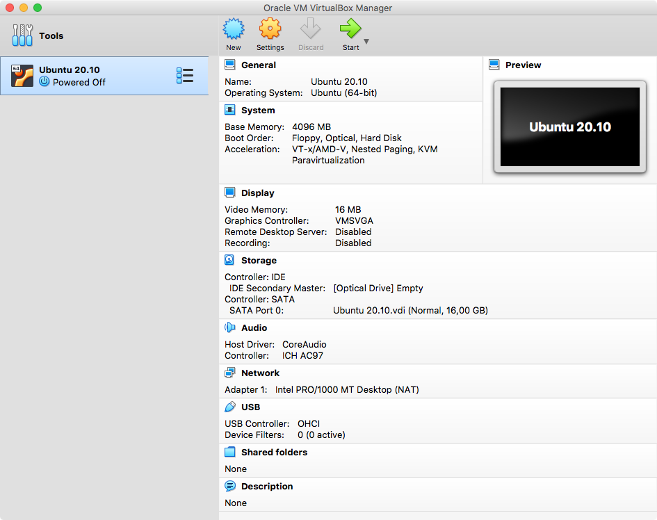
Then ensure that the ISO file is inserted into the virtual CD drive:
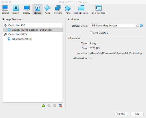
You can then boot the machine. Simply follow the instructions. Once Ubuntu is installed, we can proceed with the installation of PostgreSQL itself.
To download PostgreSQL, we suggest checking out the official PostgreSQL website. Those PostgreSQL packages provided by the community are high quality and we recommend using them for your deployment: https://www.postgresql.org/download/
Please select your desired operating system. In our example, I have selected the latest version of Ubuntu (20.10). The following steps are now necessary to install PostgreSQL:
The first thing you have to do is to add the repository to your Ubuntu installation. Here is how it works:
|
1 2 |
hans@cybertec:~# sudo sh -c 'echo 'deb http://apt.postgresql.org/pub/repos/apt $(lsb_release - cs)-pgdg main' > /etc/apt/sources.list.d/pgdg.list' |
Then you can add the keys to the system to make sure the repository is trustworthy:
|
1 2 3 |
hans@cybertec:~# wget --quiet -O - https://www.postgresql.org/media/keys/ACCC4CF8.asc | sudo apt-key add - Warning: apt-key is deprecated. Manage keyring files in trusted.gpg.d instead (see apt-key(8)). OK |
Next, we can update the package list and ensure that our system has the latest stuff:
|
1 2 3 4 5 6 7 8 9 |
hans@cybertec:~# apt-get update Hit:1 http://at.archive.ubuntu.com/ubuntu groovy InRelease Hit:2 http://at.archive.ubuntu.com/ubuntu groovy-updates InRelease Hit:3 http://at.archive.ubuntu.com/ubuntu groovy-backports InRelease Get:4 http://apt.postgresql.org/pub/repos/apt groovy-pgdg InRelease [16,8 kB] Hit:5 http://security.ubuntu.com/ubuntu groovy-security InRelease Get:6 http://apt.postgresql.org/pub/repos/apt groovy-pgdg/main amd64 Packages [162 kB] Fetched 178 kB in 1s (228 kB/s) Reading package lists... Done |
Once the repositories are ready to use, we can actually go and install PostgreSQL on our Ubuntu server.
Basically, all we need to do is run “apt-get -y install postgresql” This will automatically deploy the latest version of PostgreSQL. If we want to deploy, say, PostgreSQL 12 instead of the current PostgreSQL, we would use “apt-get install postgresql-12” instead.
Now let’s install PostgreSQL 13:
|
1 2 3 4 5 6 7 8 9 10 11 12 13 14 15 16 17 18 19 20 21 22 23 24 25 26 27 28 29 30 31 32 33 34 35 36 37 38 39 40 41 42 43 44 45 46 47 48 49 50 51 52 53 54 55 56 57 58 59 60 61 62 63 |
hans@cybertec:~# sudo apt-get -y install postgresql Reading package lists... Done Building dependency tree Reading state information... Done The following additional packages will be installed: libpq5 pgdg-keyring postgresql-13 postgresql-client-13 postgresql-client-common postgresql-common sysstat Suggested packages: postgresql-doc postgresql-doc-13 libjson-perl isag The following NEW packages will be installed: libpq5 pgdg-keyring postgresql postgresql-13 postgresql-client-13 postgresql-client-common postgresql-common sysstat 0 upgraded, 8 newly installed, 0 to remove and 150 not upgraded. Need to get 17,7 MB of archives. After this operation, 59,2 MB of additional disk space will be used. Get:1 http://at.archive.ubuntu.com/ubuntu groovy/main amd64 sysstat amd64 12.4.0-1 [471 kB] Get:2 http://apt.postgresql.org/pub/repos/apt groovy-pgdg/main amd64 libpq5 amd64 13.1-1.pgdg20.10+1 [175 kB] Get:3 http://apt.postgresql.org/pub/repos/apt groovy-pgdg/main amd64 pgdg-keyring all 2018.2 [10,7 kB] ... Creating config file /etc/postgresql-common/createcluster.conf with new version Building PostgreSQL dictionaries from installed myspell/hunspell packages... en_us Removing obsolete dictionary files: apt-get -y install postgresql Created symlink /etc/systemd/system/multi-user.target.wants/postgresql.service → /lib/systemd/system/postgresql.service. Setting up postgresql-13 (13.1-1.pgdg20.10+1) ... Creating new PostgreSQL cluster 13/main ... /usr/lib/postgresql/13/bin/initdb -D /var/lib/postgresql/13/main --auth-local peer --auth-host md5 The files belonging to this database system will be owned by user 'postgres'. This user must also own the server process. The database cluster will be initialized with locales COLLATE: en_US.UTF-8 CTYPE: en_US.UTF-8 MESSAGES: en_US.UTF-8 MONETARY: de_AT.UTF-8 NUMERIC: de_AT.UTF-8 TIME: de_AT.UTF-8 The default database encoding has accordingly been set to 'UTF8'. The default text search configuration will be set to 'english'. Data page checksums are disabled. fixing permissions on existing directory /var/lib/postgresql/13/main ... ok creating subdirectories ... ok selecting dynamic shared memory implementation ... posix selecting default max_connections ... 100 selecting default shared_buffers ... 128MB selecting default time zone ... Europe/Vienna creating configuration files ... ok running bootstrap script ... ok performing post-bootstrap initialization ... ok syncing data to disk ... ok Success. You can now start the database server using: pg_ctlcluster 13 main start Ver Cluster Port Status Owner Data directory Log file 13 main 5432 down postgres /var/lib/postgresql/13/main /var/log/postgresql/postgresql-13-main.log update-alternatives: using /usr/share/postgresql/13/man/man1/postmaster.1.gz to provide /usr/share/man/man1/postmaster.1.gz (postmaster.1.gz) in auto mode Setting up postgresql (13+223.pgdg20.10+1) ... ... |
The beauty of this setup is that everything was done automatically by the packages. This includes but is not limited to:
systemd configurationNow, all that remains to be done is to enable the services to ensure that the database is running correctly and automatically - in case the system is restarted.
Enabling the service is easy and can be done using the standard systemd procedure. Basically the service should already be active but it makes sense to double check to make sure that stuff is really enabled:
|
1 2 3 |
hans@cybertec:~# sudo systemctl enable postgresql Synchronizing state of postgresql.service with SysV service script with /lib/systemd/systemd-sysv-install. Executing: /lib/systemd/systemd-sysv-install enable postgresql |
Once the service has been enabled, we can start the instance so that we can use it directly, without a restart:
|
1 |
hans@cybertec:~# sudo systemctl start postgresql |
Ubuntu did not issue any errors. However, it is usually a good idea to check if the database is indeed running. There are two ways to do that:
pg_isready to check the systemFirst, let’s check the process table:
|
1 2 3 4 5 6 7 8 9 |
hans@cybertec:~# ps axf | grep postgres 58406 pts/2 S+ 0:00 _ grep --color=auto postgres 47883 ? Ss 0:00 /usr/lib/postgresql/13/bin/postgres -D /var/lib/postgresql/13/main -c config_file=/etc/postgresql/13/main/postgresql.conf 47885 ? Ss 0:00 _ postgres: 13/main: checkpointer 47886 ? Ss 0:00 _ postgres: 13/main: background writer 47887 ? Ss 0:00 _ postgres: 13/main: walwriter 47888 ? Ss 0:00 _ postgres: 13/main: autovacuum launcher 47889 ? Ss 0:00 _ postgres: 13/main: stats collector 47890 ? Ss 0:00 _ postgres: 13/main: logical replication launcher |
The second option is to use pg_isready:
|
1 2 3 4 5 |
hans@cybertec:~# su - postgres postgres@cybertec:~$ pg_isready /var/run/postgresql:5432 - accepting connections postgres@cybertec:~$ pg_isready -V pg_isready (PostgreSQL) 13.1 (Ubuntu 13.1-1.pgdg20.10+1) |
Switch to the “postgres” user, and then call pg_isready. If you want a little bit more information, you can also add the -V (verbose) flag to the end. The beauty is that pg_isready returns a POSIX compliant return code, so you can easily use it in your scripts.
After we have installed and enabled PostgreSQL on our Ubuntu system, we can check which databases there are:
|
1 2 3 4 5 6 7 8 9 10 |
postgres@cybertec:~$ psql -l List of databases Name | Owner | Encoding | Collate | Ctype | Access privileges -----------+----------+----------+-------------+-------------+----------------------- postgres | postgres | UTF8 | en_US.UTF-8 | en_US.UTF-8 | template0 | postgres | UTF8 | en_US.UTF-8 | en_US.UTF-8 | =c/postgres + | | | | | postgres=CTc/postgres template1 | postgres | UTF8 | en_US.UTF-8 | en_US.UTF-8 | =c/postgres + | | | | | postgres=CTc/postgres (3 rows) |
“psql -l” connects to the database and lists the databases in our PostgreSQL cluster. This works perfectly - so we can already log in, and easily create a new database:
|
1 2 3 4 5 6 7 |
postgres@cybertec:~$ psql postgres psql (13.1 (Ubuntu 13.1-1.pgdg20.10+1)) Type 'help' for help. postgres=# CREATE DATABASE test; CREATE DATABASE postgres=# c test You are now connected to database 'test' as user 'postgres' |
PostgreSQL is now ready for action. You can already go ahead and use the system according to your needs. If you want to tune your database and find good configuration parameters, we recommend checking out the PostgreSQL configuration tool (pgconfigurator). It will help you to achieve better performance by adjusting some key parameters in the postgresql.conf configuration file.
If you want to improve your database setup even more, we recommend checking out a way to cluster PostgreSQL to achieve higher availability. We have compiled a post for you showing how HA can easily be achieved. Check it out.