Since my last article about MobilityDB, the overall project has further developed and improved.
This is a very good reason to invest some time and showcase MobilityDB’s rich feature stack by analyzing historical flight data from OpenSky-Network, a non-profit organisation which has been collecting air traffic surveillance data since 2013.
Table of Contents
From data preparation and data visualization to analysis – this article covers all the steps needed to quick-start analyzing spatio-temporal data with PostGIS and MobilityDB together.
For a basic introduction to MobilityDB, please check out previous MobilityDB post first.
The article is divided into four sections:
First, you need a current PostgreSQL database, equipped with PostGIS and MobilityDB. I recommend using the latest releases available for your OS of choice, even though MobilityDB works with older releases of PostgreSQL and PostGIS, too. Alternatively, use a docker container from https://registry.hub.docker.com/r/codewit/mobilitydb for those who don’t want to build MobilityDB from scratch.
Second, you'll need a tool to copy our raw flight data served as huge csv files to our database. For this kind of task, I typically use ogr2ogr, a command-line tool shipped with gdal.
Lastly, to visualize our results graphically, we’ll utilize our good old friend “Quantum GIS”, a feature-rich GIS-client, which is available for various operating systems.
The foundation of our analysis is historical flight data, offered by OpenSky-Network free of charge for non-commercial usage. OpenSky offers snapshots of the previous Monday's complete state vector data for the last 6 months. These data sets cover information about time (update interval is one second), icao24, lat/lon, velocity, heading, vertrate, callsign, onground, alert/spi, squawk, baro/geoaltitude, lastposupdate and lastcontact. A detailed description can be found at here.
Enough theory; let’s start by downloading historical datasets for our analysis. The foundation for this post are 24 csv files covering flight data for the day 2022-02-28, which can be downloaded from here.
We’ll continue by creating a new PostgreSQL database, with extensions for PostGIS and MobilityDB enabled. The database will store our state vectors.
|
1 2 3 4 5 6 7 8 9 10 11 12 13 14 15 16 17 |
postgres=# create database flightanalysis; CREATE DATABASE postgres=# c flightanalysis You are now connected to database 'flightanalysis' as user 'postgres'. flightanalysis=# create extension MobilityDB cascade; NOTICE: installing required extension 'postgis' CREATE EXTENSION flightanalysis=# dx List of installed extensions Name | Version | Schema | Description ------------+---------+------------+------------------------------------------------------------ mobilitydb | 1.0.0 | public | MobilityDB Extension plpgsql | 1.0 | pg_catalog | PL/pgSQL procedural language postgis | 3.2.1 | public | PostGIS geometry and geography spatial types and functions (3 rows) |
From OpenSky’s dataset descriptions, we inherit a data structure for a staging table, which stores unaltered raw state vectors.
|
1 2 3 4 5 6 7 8 9 10 11 12 13 14 15 16 17 18 19 20 21 22 23 24 25 26 |
create table tvectors ( ogc_fid integer default nextval('flightsegments_ogc_fid_seq'::regclass) not null constraint flightsegments_pkey primary key, time integer, ftime timestamp with time zone, icao24 varchar, lat double precision, lon double precision, velocity double precision, heading double precision, vertrate double precision, callsign varchar, onground boolean, alert boolean, spi boolean, squawk integer, baroaltitude double precision, geoaltitude double precision, lastposupdate double precision, lastcontact double precision ); create index idx_points_icao24 on tvectors (icao24, callsign); |
From a directory containing the uncompressed csv files, state vectors can now be imported to our flightanalysis database as follows:
for f in ls *.csv; do
ogr2ogr -f PostgreSQL PG:"user=postgres dbname=flightanalysis" $f -oo AUTODETECT_TYPE=YES -nln tvectors --config PG_USE_COPY YES
done
flightanalysis=# select count(*) from tvectors;
count
--------------
52261548
(1 row)
To analyse our vectors with MobilityDB, we must now turn our native position data into trajectories.
MobilityDB offers various data types to model trajectories, such as tgeompoint, which represents a temporal geometry point type.
|
1 2 3 4 5 6 7 8 9 10 11 12 13 14 15 |
create table if not exists flightsegments ( icao24 varchar not null, callsign varchar not null, trip tgeompoint, traj geometry(Geometry,4326), constraint flightsegment_2_pkey primary key (icao24, callsign) ); create index idx_trip on flightsegments using gist (trip); create index idx_traj on flightsegments using gist (traj); |
To track individual flights from airplanes, trajectories must be generated by selecting vectors by icao24 and callsign ordered by time.
Initially, timestamps (column time) are represented as a unix timestamp in our staging table. For ease of use, we’ll translate unix timestamps to timestamps with time zones first.
|
1 2 3 4 5 |
update tvectors set ftime= to_timestamp(time) AT TIME ZONE 'UTC'; create index idx_points_ftime on tvectors (ftime); |
Finally, we can create our trajectories by aggregating locations by icao24 and callsign ordered by time.
|
1 2 3 4 5 6 7 8 |
insert into flightsegments(icao24, callsign, trip) SELECT icao24, callsign, tgeompoint_seq(array_agg(tgeompoint_inst(ST_SetSRID(ST_MakePoint(Lon, Lat), 4326), ftime) ORDER BY ftime)) from tvectors where lon is not null and lat is not null group by icao24, callsign; |
To visualize our aggregated vectors in QGIS, someone must extract the vectors’ raw geometries from tgeompoint, as this data type is not supported natively out of the box from QGIS.
To create a geometrically simplified version for better performance, we’ll utilize st_simplify on top of trajectory. It’s worth mentioning that simplification methods from MobilityDB also exist, which simplify the whole trajectory and not only its geometry.
|
1 2 |
update flightsegments set traj = st_simplify(trajectory(trip)::geometry, 0.001)::geometry; |
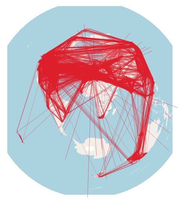
From the images below, you can see the vast number of vectors these freely available datasets contain just for one single day.
You can see in the image that the data is noisy, and must be further cleaned and filtered. Gaps in coverage and recording lead to trajectories spanning the world - and subsequently lead to wrong and misleading results. Nevertheless, we’ll skip this extensive cleansing step today (but might cover this as a separate blog post) and move on with our analysis focusing on a rather small area.
Let’s investigate the trajectories and play through some interesting scenarios.
|
1 2 |
select count(distinct icao24) from flightsegments; |
|
1 2 3 4 5 |
flightanalysis=# select count(distinct icao24) from flightsegments; count ------- 41663 (1 row) |
|
1 2 3 4 5 |
flightanalysis=# select avg(duration(trip)) from flightsegments where st_length(trajectory(trip::tgeogpoint)) > 0; avg ----------------- 03:50:48.245525 (1 row) |
For this kind of analysis, download and import country borders from Natural Earth first.
|
1 2 3 4 5 6 7 8 9 10 |
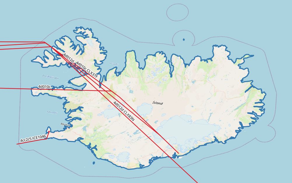
select icao24, callsign, trajectory(atPeriod(T.Trip, '[2022-02-28 00:00:00+00, [2022-2-28 03:00:00+00]'::period)) FROM flightsegments T, ne_10m_admin_0_countries R WHERE T.Trip && stbox(R.geom, '[2022-02-28 00:00:00+00, [2022-02-28 03:00:00+00]'::period) AND st_intersects(trajectory(atPeriod(T.Trip, '[2022-02-28 00:00:00+00, [2022-2-28 03:00:00+00]'::period)), r.geom) and R.name = 'Iceland' and st_length(trajectory(atPeriod(T.Trip, '[2022-02-28 00:00:00+00, [2022-2-28 03:00:00+00]'::period))::geography) > 0 |
|
1 2 3 4 5 6 7 8 9 10 11 12 13 14 15 16 17 18 19 |
select icao24, callsign, (duration( (atgeometry((atPeriod(T.Trip::tgeompoint, '[2022-02-28 00:00:00+00, [2022-02-28 03:00:00+00]'::period)), R.geom))))::varchar, trajectory( atgeometry((atPeriod(T.Trip::tgeompoint, '[2022-02-28 00:00:00+00, [2022-02-28 03:00:00+00]'::period)), R.geom)) FROM flightsegments T, ne_10m_admin_0_countries R WHERE T.Trip && stbox(R.geom, '[2022-02-28 00:00:00+00, [2022-02-28 03:00:00+00]'::period) AND st_intersects(trajectory(atPeriod(T.Trip, '[2022-02-28 00:00:00+00, [2022-2-28 03:00:00+00]'::period)), r.geom) and R.name = 'Iceland' and st_length(trajectory(atPeriod(T.Trip, '[2022-02-28 00:00:00+00, [2022-2-28 03:00:00+00]'::period))::geography) > 0 |
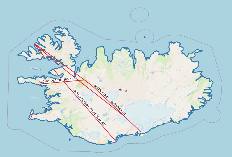
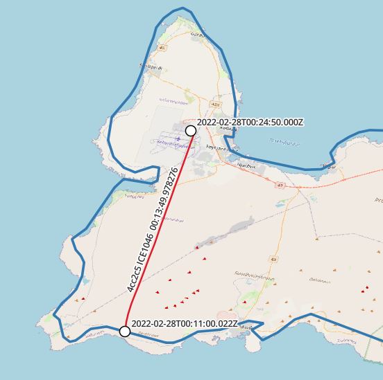
Note that in this case, the plane did not leave the country during this trip.
|
1 2 3 4 5 6 7 8 9 10 11 12 13 14 15 16 17 18 19 20 21 22 23 24 25 26 27 |
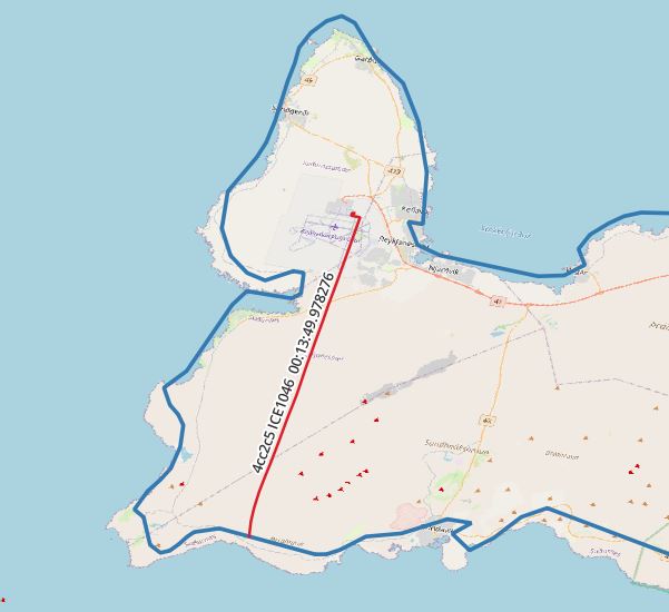
with segments as ( select icao24, callsign, unnest(sequences( atgeometry( (atPeriod(T.Trip::tgeompoint, '[2022-02-28 00:00:00+00, [2022-02-28 03:00:00+00]'::period)), R.geom))) segment FROM flightsegments T, ne_10m_admin_0_countries R WHERE T.Trip && stbox(R.geom, '[2022-02-28 00:00:00+00, [2022-02-28 03:00:00+00]'::period) AND st_intersects(trajectory(atPeriod(T.Trip, '[2022-02-28 00:00:00+00, [2022-2-28 03:00:00+00]'::period)), r.geom) and R.name = 'Iceland' and trim(callsign) = 'ICE1046' and st_length(trajectory(atPeriod(T.Trip, '[2022-02-28 00:00:00+00, [2022-2-28 03:00:00+00]'::period))::geography) > 0) select icao24,callsign, st_startpoint(getvalues(segment)), st_endpoint(getvalues(segment)), starttimestamp(segment), endtimestamp(segment) from segments |
MobilityDB’s rich feature stack drastically simplifies analysis on spatio-temporal data. If I may be allowed to imagine further uses for it, various businesses come to my mind where it could be applied in a smart and efficient manner. Toll systems, surveillance, logistics - just to name a few. Finally, its upcoming release will pave the way for new usages, from research and test utilization to production scenarios.
I hope you enjoyed this session. Learn more about using PostGIS by checking out my blog on spatial datasets based on the OpenStreetMap service
In case you want to learn more about PostGIS and Mobility, just get in touch with the folks from CYBERTEC. Stay tuned!
Noice! Thanks for your work done
Thank you very much for your great work.
I have a few queries:
1. How to use velocity, heading and altitude fields to precisely depict/present the flights on map.
2. What sort of different analysis can be drawn from this type of data?
Would you please guide about it?
Thanks for this, MobilityDB has great features but the documentation is not that great.