UPDATED July 2023: EXPLAIN ANALYZE is the key to optimizing SQL statements in PostgreSQL. This article does not attempt to explain everything there is to it. Rather, I want to give you a brief introduction, explain what to look for and show you some helpful tools to visualize the output.
Also, I want to call your attention to a new patch I wrote which has been included in PostgreSQL 16, EXPLAIN GENERIC PLAN. You can read about it here.
EXPLAIN ANALYZE?If you have an SQL statement that executes too slowly, you want to know what is going on and how to fix it. In SQL, it is harder to see how the engine spends its time, because it is not a procedural language, but a declarative language: you describe the result you want to get, not how to calculate it. The EXPLAIN command shows you the execution plan that is generated by the optimizer. This is helpful, but typically you need more information.
You can obtain such additional information by adding EXPLAIN options in parentheses.
EXPLAIN optionsANALYZE: with this keyword, EXPLAIN does not only show the plan and PostgreSQL's estimates, but it also executes the query (so be careful with UPDATE and DELETE!) and shows the actual execution time and row count for each step. This is indispensable for analyzing SQL performance.BUFFERS: You can only use this keyword together with ANALYZE, and it shows how many 8kB-blocks each step reads, writes and dirties. You always want this.VERBOSE: if you specify this option, EXPLAIN shows all the output expressions for each step in an execution plan. This is usually just clutter, and you are better off without it, but it can be useful if the executor spends its time in a frequently-executed, expensive function.SETTINGS: this option exists since v12 and includes all performance-relevant parameters that are different from their default value in the output.WAL: introduced in v13, this option shows the WAL usage incurred by data modifying statements. You can only use it together with ANALYZE. This is always useful information!FORMAT: this specifies the output format. The default format TEXT is the best for humans to read, so use that to analyze query performance. The other formats (XML, JSON and YAML are better for automated processing.Typically, the best way to call EXPLAIN is:
|
1 |
EXPLAIN (ANALYZE, BUFFERS) /* SQL statement */; |
Include SETTINGS if you are on v12 or better and WAL for data modifying statements from v13 on.
It is highly commendable to set track_io_timing = on to get data about the I/O performance.
You cannot use EXPLAIN for all kinds of statements: it only supports SELECT, INSERT, UPDATE, DELETE, EXECUTE (of a prepared statement), CREATE TABLE ... AS and DECLARE (of a cursor).
Note that EXPLAIN ANALYZE adds a noticeable overhead to the query execution time, so don't worry if the statement takes longer.
There is always a certain variation in query execution time, as data may not be in cache during the first execution. That's why it is valuable to repeat EXPLAIN ANALYZE a couple of times and see if the result changes.
EXPLAIN ANALYZE?PostgreSQL displays some of the information for each node of the execution plan, and you see some of it in the footer.
EXPLAIN without optionsPlain EXPLAIN will give you the estimated cost, the estimated number of rows and the estimated size of the average result row. The unit for the estimated query cost is artificial (1 is the cost for reading an 8kB page during a sequential scan). There are two cost values: the startup cost (cost to return the first row) and the total cost (cost to return all rows).
|
1 2 3 4 5 6 7 8 |
EXPLAIN SELECT count(*) FROM c WHERE pid = 1 AND cid > 200; QUERY PLAN ------------------------------------------------------------ Aggregate (cost=219.50..219.51 rows=1 width=8) -> Seq Scan on c (cost=0.00..195.00 rows=9800 width=0) Filter: ((cid > 200) AND (pid = 1)) (3 rows) |
ANALYZE optionANALYZE gives you a second parenthesis with the actual execution time in milliseconds, the actual row count and a loop count that shows how often that node was executed. It also shows the number of rows that filters have removed.
|
1 2 3 4 5 6 7 8 9 10 11 |
EXPLAIN (ANALYZE) SELECT count(*) FROM c WHERE pid = 1 AND cid > 200; QUERY PLAN --------------------------------------------------------------------------------------------------------- Aggregate (cost=219.50..219.51 rows=1 width=8) (actual time=4.286..4.287 rows=1 loops=1) -> Seq Scan on c (cost=0.00..195.00 rows=9800 width=0) (actual time=0.063..2.955 rows=9800 loops=1) Filter: ((cid > 200) AND (pid = 1)) Rows Removed by Filter: 200 Planning Time: 0.162 ms Execution Time: 4.340 ms (6 rows) |
In the footer, you see how long PostgreSQL took to plan and execute the query. You can suppress that information with SUMMARY OFF.
BUFFERS optionThis option shows how many data blocks were found in the cache (hit) for each node, how many had to be read from disk, how many were written and how many dirtied. In recent versions, the footer contains the same information for the work done by the optimizer, if it didn't find all its data in the cache.
If track_io_timing = on, you will get timing information for all I/O operations.
|
1 2 3 4 5 6 7 8 9 10 11 12 13 14 15 16 17 18 |
EXPLAIN (ANALYZE, BUFFERS) SELECT count(*) FROM c WHERE pid = 1 AND cid > 200; QUERY PLAN --------------------------------------------------------------------------------------------------------- Aggregate (cost=219.50..219.51 rows=1 width=8) (actual time=2.808..2.809 rows=1 loops=1) Buffers: shared read=45 I/O Timings: read=0.380 -> Seq Scan on c (cost=0.00..195.00 rows=9800 width=0) (actual time=0.083..1.950 rows=9800 loops=1) Filter: ((cid > 200) AND (pid = 1)) Rows Removed by Filter: 200 Buffers: shared read=45 I/O Timings: read=0.380 Planning: Buffers: shared hit=48 read=29 I/O Timings: read=0.713 Planning Time: 1.673 ms Execution Time: 3.096 ms (13 rows) |
EXPLAIN ANALYZE outputYou see that you end up with quite a bit of information even for simple queries. To extract meaningful information, you have to know how to read it.
First, you have to understand that a PostgreSQL execution plan is a tree structure consisting of several nodes. The top node (the Aggregate above) is at the top, and lower nodes are indented and start with an arrow (->). Nodes with the same indentation are on the same level (for example, the two relations combined with a join).
PostgreSQL executes a plan top down, that is, it starts with producing the first result row for the top node. The executor processes lower nodes “on demand”, that is, it fetches only as many result rows from them as it needs to calculate the next result of the upper node. This influences how you have to read “cost” and “time”: the startup time for the upper node is at least as high as the startup time of the lower nodes, and the same holds for the total time. If you want to find the net time spent in a node, you have to subtract the time spent in the lower nodes. Parallel queries make that even more complicated.
On top of that, you have to multiply the cost and the time with the number of “loops” to get the total time spent in a node.
EXPLAIN ANALYZE outputEXPLAIN ANALYZE outputSince reading a longer execution plan is quite cumbersome, there are a few tools that attempt to visualize this “sea of text”:
EXPLAIN ANALYZE visualizerThis tool can be found at https://explain.depesz.com/. If you paste the execution plan in the text area and hit “Submit”, you will get output like this:
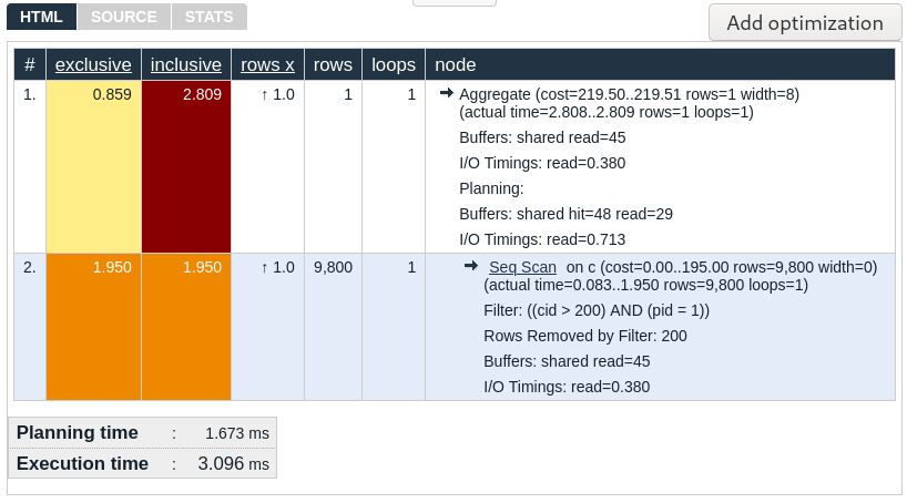
The execution plan looks somewhat similar to the original, but optically more pleasing. There are useful additional features:
What I particularly like about this tool is that all the original EXPLAIN text is right there for you to see, once you have focused on an interesting node. The look and feel is decidedly more “old school” and no-nonsense, and this site has been around for a long time.
EXPLAIN ANALYZE visualizerThis tool can be found at https://explain.dalibo.com/. Again, you paste the raw execution plan and hit “Submit”. The output is presented as a tree:
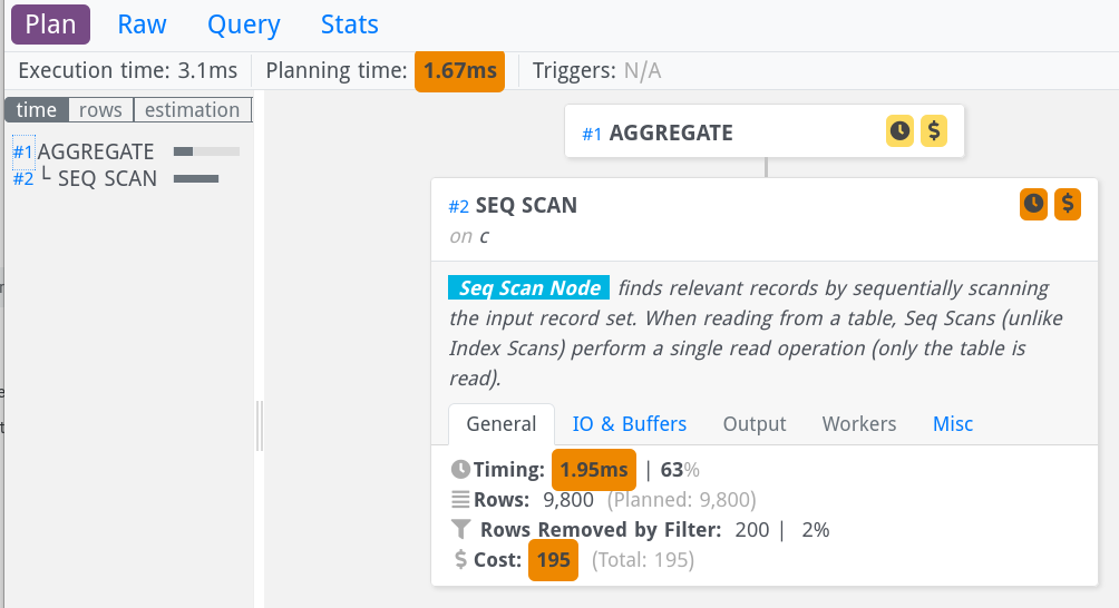
Initially, the display hides the details, but you can show them by clicking on a node, like I have done with the second node in the image above. On the left, you see a small overview over all nodes, and from there you can jump to the right side to get details. Features that add value are:
The nice thing about this tool is that it makes the tree structure of the execution plan clearly visible. The look and feel is more up-to-date. On the downside, it hides the detailed information somewhat, and you have to learn where to search for it.
EXPLAIN (ANALYZE, BUFFERS) (with track_io_timing turned on) will show you everything you need to know to diagnose SQL statement performance problems. To keep from drowning in a sea of text, you can use Depesz' or Dalibo's visualizer. Both provide roughly the same features.
For more information on detailed query performance analysis, see my blog about using EXPLAIN(ANALYZE) with parameterized statements.
Before you can start tuning queries, you have to find the ones that use most of your server's resources. Here is an article that describes how you can use pg_stat_statements to do just that.
In order to receive regular updates on important changes in PostgreSQL, subscribe to our newsletter, or follow us on Twitter, Facebook, or LinkedIn.
Bulk loading is the quickest way to import large amounts of data into a PostgreSQL database. There are various ways to facilitate large-scale imports, and many different ways to scale are also available. This post will show you how to use some of these tricks, and explain how fast importing works. You can use this knowledge to optimize data warehousing or any other data-intensive workload.
There are several things to take into consideration in order to speed up bulk loading of massive amounts of data using PostgreSQL:
Let us take a look at these things in greater detail.
The first thing to consider is that COPY is usually a LOT better than plain inserts. The reason is that INSERT has a lot of overhead. People often ask: What kind of overhead is there? What makes COPY so much faster than INSERT? There are a variety of reasons: In the case of INSERT, every statement has to check for locks, check for the existence of the table and the columns in the table, check for permissions, look up data types and so on. In the case of COPY, this is only done once, which is a lot faster. Whenever you want to write large amounts of data, data COPY is usually the way to go.
To show what kind of impact this change has in terms of performance, I have compiled a short example.
Let’s create a table as well as some sample data:
|
1 2 3 4 5 6 7 8 |
test=# CREATE TABLE t_sample ( a varchar(50), b int, c varchar(50), d int ); CREATE TABLE |
The sample table consists of 4 columns which is pretty simple.
In the next step, we will compile a script containing 1 million INSERT statements in a single transaction:
|
1 2 3 4 5 6 |
BEGIN; INSERT INTO t_sample VALUES ('abcd', 1, 'abcd', 1); INSERT INTO t_sample VALUES ('abcd', 1, 'abcd', 1); INSERT INTO t_sample VALUES ('abcd', 1, 'abcd', 1); … COMMIT; |
Running the script can be done using psql:
|
1 2 3 4 5 |
iMac:~ hs$ time psql test < /tmp/sample.sql > /dev/null real 1m20.883s user 0m11.515s sys 0m10.070s |
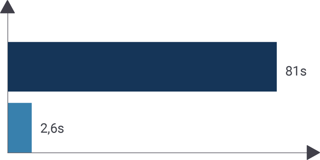
We need around 81 seconds to run this simple test, which is A LOT of time. Single INSERT statements are therefore obviously not the solution to perform quick imports and efficient bulk loading.
As I have already mentioned, COPY is a lot more efficient than INSERT, so let’s use the same data, but feed it to COPY instead;
|
1 2 3 4 5 6 7 |
COPY t_sample FROM stdin; abcd 1 abcd 1 abcd 1 abcd 1 abcd 1 abcd 1 abcd 1 abcd 1 … . |
Running the script is again an easy thing to do:
|
1 2 3 4 5 |
iMac:~ hs$ time psql test < /tmp/bulk.sql > /dev/null real 0m2.646s user 0m0.110s sys 0m0.043s |
Keep in mind that I have executed this test on a fairly old machine, on a totally untuned database. On modern hardware and on a more modern operating system, a lot more can be achieved than on my local iMac desktop machine. Loading 1 million lines or more is not uncommon in the real world. Of course, this data depends on the length of a “record” and so on. However, it is important to get a feeling for what is possible and what is not.
NOTE: Runtimes might vary. This has many reasons. One of them is certainly related to the hardware in use here. We have seen that many SSDs provide us with quite unstable response times.
The PostgreSQL configuration does have an impact on bulk loading performance. There are many configuration parameters which are vital to database performance, and loading in particular. However, I explicitly want to focus your attention on checkpoint and I/O performance. If you want to load billions of rows, I/O is king. There are various angles to approach the topic:
The following settings are important:
Setting this value to 100 or 200 GB in case of bulk-load intense workloads is definitely not out of scope.
Keep in mind that increased checkpoint distances DO NOT put your server at risk. It merely affects the way PostgreSQL writes data. Also keep in mind that more disk space will be consumed and recovery might take longer, in case of a crash.
If you want to learn more about checkpointing, check out this article about reducing the amount of WAL written.
However, what if there were a way to get rid of WAL altogether? Well, there is one. It is called an “unlogged table”. What is the general idea? Often we got the following sequence of events:
This is the ideal scenario to use the WAL bypass provided by unlogged tables:
|
1 2 3 4 5 6 7 8 9 10 11 12 13 14 15 16 17 18 |
test=# DROP TABLE t_sample ; DROP TABLE test=# CREATE UNLOGGED TABLE t_sample ( a varchar(50), b int, c varchar(50), d int ); CREATE TABLE test=# d t_sample Unlogged table 'public.t_sample' Column | Type | Collation | Nullable | Default --------+-----------------------+-----------+----------+--------- a | character varying(50) | | | b | integer | | | c | character varying(50) | | | d | integer | | | |
Let’s load the same data again:
|
1 2 3 4 5 6 7 8 9 10 11 |
iMac:~ hs$ time psql test < /tmp/sample.sql > /dev/null real 0m59.296s user 0m10.597s sys 0m9.417s iMac:~ hs$ time psql test < /tmp/bulk.sql > /dev/null real 0m0.618s user 0m0.107s sys 0m0.038s |
As you can see, the entire thing is a lot faster. 81 seconds vs. 59 seconds and 2.6 vs. 0.6 seconds. The difference is massive.
The reason is that an unlogged table does not have to write the data twice (no WAL needed). However, this comes with a price tag attached to it:
These restrictions imply that an unlogged table is not suitable for storing “normal” data. However, it is ideal for staging areas and bulk loading.
Tables can be made logged and unlogged. Many people expect these to be cheap operations but this is not true.
|
1 2 3 4 5 6 7 8 9 10 11 12 13 14 |
test=# SELECT pg_current_wal_lsn(); pg_current_wal_lsn -------------------- 5/3AC7CCD0 (1 row) test=# ALTER TABLE t_sample SET LOGGED; ALTER TABLE test=# SELECT pg_current_wal_lsn(); pg_current_wal_lsn -------------------- 5/3F9048A8 (1 row) |
In addition to setting the table from UNLOGGED to LOGGED, I have measured the current WAL position.
What we can see is that a lot of data has been written:
|
1 2 3 4 5 6 7 |
test=# SELECT '5/3F9048A8'::pg_lsn - '5/3AC7CCD0'::pg_lsn; ?column? ----------- 80247768 (1 row) Time: 11.298 ms |
Wow, we have produced 80 MB of WAL (if you do exactly one COPY on an empty table - the amount will grow if you run more imports). In case of COPY + INSERT, the volume will be a lot higher.
From this, we draw the conclusion that if we want to do efficient bulk loading setting a table from LOGGED to UNLOGGED, importing the data and setting it back to LOGGED might not be the best of all ideas - because as soon as a table is set back to LOGGED, the entire content of the table has to be sent to the WAL, to make sure that the replicas can receive the content of the table.
|
1 2 3 4 5 6 7 8 9 10 11 12 13 14 15 16 17 18 19 |
test=# SELECT count(*) FROM t_sample; count --------- 1000001 (1 row) test=# CREATE TABLE t_index (LIKE t_sample); CREATE TABLE test=# CREATE INDEX idx_a ON t_index (a); CREATE INDEX test=# CREATE INDEX idx_b ON t_index (b); CREATE INDEX test=# timing Timing is on. test=# INSERT INTO t_index SELECT * FROM t_sample; INSERT 0 1000001 Time: 8396.210 ms (00:08.396) |
It takes around 8 seconds to copy the data over. Let’s try the same thing by creating the indexes later:
|
1 2 3 4 5 6 7 8 9 10 11 12 13 14 |
test=# CREATE TABLE t_noindex (LIKE t_sample); CREATE TABLE test=# INSERT INTO t_noindex SELECT * FROM t_sample; INSERT 0 1000001 Time: 4789.017 ms (00:04.789) test=# SET maintenance_work_mem TO '1 GB'; SET Time: 13.059 ms test=# CREATE INDEX idx_aa ON t_noindex (a); CREATE INDEX Time: 1151.521 ms (00:01.152) test=# CREATE INDEX idx_bb ON t_noindex (b); CREATE INDEX Time: 1086.972 ms (00:01.087) |
We can see that the copy process (= INSERT) is a lot faster than before. In total, it is quicker to produce the index later. Also keep in mind that I am using synthetic data on Mac OSX (not too efficient) here. If you repeat the test with a lot more real data, the difference is a lot higher.
Create indexes after importing data if possible.
Triggers are also an important factor. One could say that triggers are “the natural enemy” of bulk loading performance. Let’s take a look at the following example:
|
1 2 3 4 5 6 7 8 9 10 11 12 13 14 15 16 17 18 19 20 21 |
iMac:~ hs$ head -n 20 /tmp/bulk.sql BEGIN; CREATE FUNCTION dummy() RETURNS trigger AS $ BEGIN NEW.b := NEW.b + 1; NEW.d := NEW.d + 1; RETURN NEW; END; $ LANGUAGE 'plpgsql'; CREATE TRIGGER mytrig BEFORE INSERT ON t_sample FOR EACH ROW EXECUTE PROCEDURE dummy(); COPY t_sample FROM stdin; abcd 1 abcd 1 abcd 1 abcd 1 abcd 1 abcd 1 abcd 1 abcd 1 |
Our trigger is really simple. All it does is to modify two entries in our data. However, the trigger will add an extra function call to every row, which really adds up.
In our case, we have got the following data: The variation with trigger is around 3 times slower. However, the real difference highly depends on the complexity of the trigger, the size of a row and a lot more. There is no way to state that “a trigger slows things down by a factor of X”. One has to see, case-by-case, what happens.
There is more to importing large amounts of data into PostgreSQL than meets the eye. So far, we have optimized checkpoints, touched indexes, triggers and so on. But what about the column order? Let’s try to find out.
In PostgreSQL, column order does make a real difference. It is generally a good idea to put “fixed length” columns in front. In other words: int8, int4, timestamptz and so on should be at the beginning of the table. Variable length data types such as varchar, text and so on should be at the end of the table. The reason for this is that CPU alignment is an issue on disk. This is true for normal heap tables (not for zheap).
Shrinking the size of a table without changing the content can speed things up, because it helps to avoid or reduce one of the key bottlenecks when bulk loading data: I/O. Check out this article to find out more.
If what you have seen so far is still not enough, we can recommend some tools to improve bulk loading even more. The following tools can be recommended:
Both tools are very well known and widely used. You can use them safely.
If you have further questions regarding these tools, please don’t hesitate to ask in the comment section, or send us an email.
If you want to know more about PostgreSQL performance, we also recommend checking out our consulting services. We help you to tune your database and make sure that your servers are operating perfectly.

UPDATED 14.05.2022: Sometimes customers ask me about the best choice for auto-generated primary keys. In this article, I'll explore the options and give recommendations.
Every table needs a primary key. In a relational database, it is important to be able to identify an individual table row. If you wonder why, search the internet for the thousands of questions asking for help with removing duplicate entries from a table.
You are well advised to choose a primary key that is not only unique, but also never changes during the lifetime of a table row. This is because foreign key constraints typically reference primary keys, and changing a primary key that is referenced elsewhere causes trouble or unnecessary work.
Now, sometimes a table has a natural primary key, for example the social security number of a country's citizens. But typically, there is no such attribute, and you have to generate an artificial primary key. Some people even argue that you should use an artificial primary key even if there is a natural one, but I won't go into that “holy war”.
There are two basic techniques:
A sequence is a database object whose sole purpose in life is to generate unique numbers. It does this using an internal counter that it increments.
Sequences are highly optimized for concurrent access, and they will never issue the same number twice. Still, accessing a sequence from many concurrent SQL statements could become a bottleneck, so there is the CACHE option that makes the sequence hand out several values at once to database sessions.
Sequences don't follow the normal transactional rules: if a transaction rolls back, the sequence does not reset its counter. This is required for good performance, and it does not constitute a problem. If you are looking for a way to generate a gapless sequence of numbers, a sequence is not the right choice, and you will have to resort to less efficient and more complicated techniques.
To fetch the next value from a sequence you use the nextval function like this:
|
1 |
SELECT nextval('sequence_name'); |
See the documentation for other functions to manipulate sequences.
A UUID (universally unique identifier) is a 128-bit number that is generated with an algorithm that effectively guarantees uniqueness. There are several standardized algorithms for that. In PostgreSQL, there are a number of functions that generate UUIDs:
uuid-ossp extension offers functions to generate UUIDs. Note that because of the hyphen in the name, you have to quote the name of the extension (CREATE EXTENSION "uuid-ossp";).gen_random_uuid() to generate version-4 (random) UUIDs.Note that you should always use the PostgreSQL data type uuid for UUIDs. Don't try to convert them to strings or numeric — you will waste space and lose performance.
There are four ways to define a column with automatically generated values:
DEFAULT clauseYou can use this method with sequences and UUIDs. Here are some examples:
|
1 2 3 4 5 6 7 8 9 |
CREATE TABLE has_integer_pkey ( id bigint DEFAULT nextval('integer_id_seq') PRIMARY KEY, ... ); CREATE TABLE has_uuid_pkey ( id uuid DEFAULT gen_random_uuid() PRIMARY KEY, ... ); |
PostgreSQL uses the DEFAULT value whenever the INSERT statement doesn't explicitly insert that column.
serial and bigserial pseudo-typesThis method is a shortcut for defining a sequence and setting a DEFAULT clause as above. With this method, you define a table as follows:
|
1 2 3 4 |
CREATE TABLE uses_serial ( id bigserial PRIMARY KEY, ... ); |
That is equivalent to the following:
|
1 2 3 4 5 6 7 8 9 10 |
CREATE TABLE uses_serial ( id bigint PRIMARY KEY, ... ); CREATE SEQUENCE uses_serial_id_seq OWNED BY uses_serial.id; ALTER TABLE uses_serial ALTER id SET DEFAULT nextval('uses_serial_id_seq'); |
The “OWNED BY” clause adds a dependency between the column and the sequence, so that dropping the column automatically drops the sequence.
Using serial will create an integer column, while bigserial will create a bigint column.
This is another way to use a sequence, because PostgreSQL uses sequences “behind the scenes” to implement identity columns.
|
1 2 3 4 5 |
CREATE TABLE uses_identity ( id bigint GENERATED ALWAYS AS IDENTITY PRIMARY KEY, ... ); |
There is also “GENERATED BY DEFAULT AS IDENTITY”, which is the same, except that you won't get an error message if you try to explicitly insert a value for the column (much like with a DEFAULT clause). See below for more!
You can specify sequence options for identity columns:
|
1 2 3 4 5 6 |
CREATE TABLE uses_identity ( id bigint GENERATED ALWAYS AS IDENTITY (MINVALUE 0 START WITH 0 CACHE 20) PRIMARY KEY, ... ); |
BEFORE INSERT triggersThis is similar to DEFAULT values, but it allows you to unconditionally override a value inserted by the user with a generated value. The big disadvantage of a trigger is the performance impact.
integer(serial) or bigint(bigserial) for my auto-generated primary key?You should always use bigint.
True, an integer occupies four bytes, while a bigint needs eight. But:
integer would suffice, the four wasted bytes won't matter much. Also, not every table that you designed to be small will remain small!integer, which is 2147483647. Note that that could also happen if your table contains fewer rows than that: you might delete rows, and some sequence values can get “lost” by transactions that are rolled back.integer to bigint in a big table inside an active database without causing excessive down time, so you should save yourself that pain.With bigint, you are certain to never exceed the maximum of 9223372036854775807: even if you insert 10000 rows per second without any pause, you have almost 30 million years before you reach the limit.
bigserial or an identity column for my auto-generated primary key?You should use an identity column, unless you have to support old PostgreSQL versions.
Identity columns were introduced in PostgreSQL v11, and they have two advantages over bigserial:
bigserial is proprietary PostgreSQL syntax. This will make your code more portable.GENERATED ALWAYS AS IDENTITY, you will get an error message if you try to override the generated value by explicitly inserting a number. This avoids the common problem that manually entered values will conflict with generated values later on, causing surprising application errors.So unless you have to support PostgreSQL v10 or below, there is no reason to use bigserial.
bigint or uuid for an auto-generated primary key?My advice is to use a sequence unless you use database sharding or have some other reason to generate primary keys in a "decentralized" fashion (outside a single database).
The advantages of bigint are clear:
bigint uses only eight bytes, while uuid uses 16One disadvantage of using a sequence is that it is a single object in a single database. So if you use sharding, where you distribute your data across several databases, you cannot use a sequence. In such a case, UUIDs are an obvious choice. (You could use sequences defined with an INCREMENT greater than 1 and different START values, but that might lead to problems when you add additional shards.)
Of course, if your primary key is not auto-generated by the database, but created in an application distributed across several application servers, you will also prefer UUIDs.
There are people that argue that UUIDs are better, because they spread the writes across different pages of the primary key index. That is supposed to reduce contention and lead to a more balanced or less fragmented index. The first is true, but that may actually be a disadvantage, because it requires the whole index to be cached for good performance. The second is definitely wrong, since B-tree indexes are always balanced. Also, a change in PostgreSQL v11 made sure that monotonically increasing values will fill an index more efficiently than random inserts ever could (but subsequent deletes will of course cause fragmentation). In short, any such advantages are either marginal or non-existent, and they are more than balanced by the fact that uuid uses twice as much storage, which will make the index bigger, causing more writes and occupying more of your cache.
People have argued (see for example the comments below) that sequence-generated primary keys can leak information, because they allow you to deduce the approximate order on which rows were inserted into a table. That is true, even though I personally find it hard to imagine a case where this is a real security problem. However, if that worries you, use UUIDs and stop worrying!
bigint versus uuidMy co-worker Kaarel ran a small performance test a while ago and found that uuid was slower than bigint when it came to bigger joins.
I decided to run a small insert-only benchmark with these two tables:
|
1 2 3 4 5 6 7 |
CREATE UNLOGGED TABLE test_bigint ( id bigint GENERATED ALWAYS AS IDENTITY (CACHE 200) PRIMARY KEY ); CREATE UNLOGGED TABLE test_uuid ( id uuid DEFAULT gen_random_uuid() PRIMARY KEY ); |
I performed the benchmark on my laptop (SSD, 8 cores) with a pgbench custom script that had 6 concurrent clients repeatedly run transactions of 1000 prepared INSERT statements for five minutes:
|
1 |
INSERT INTO test_bigint /* or test_uuid */ DEFAULT VALUES; |
bigint |
uuid |
|
| inserts per second | 107090 | 74947 |
| index growth per row | 30.5 bytes | 41.7 bytes |
Using bigint clearly wins, but the difference is not spectacular.
Numbers generated by a sequence and UUIDs are both useful as auto-generated primary keys.
Use identity columns unless you need to generate primary keys outside a single database, and make sure all your primary key columns are of type bigint.
If you are interested in reading more about primary keys, see also Hans' post on Primary Keys vs. Unique Constraints.
In other news, in PostgreSQL 15 default permissions for the public schema were modified, which can cause errors.
Find out more about this important change here.
In order to receive regular updates on important changes in PostgreSQL, subscribe to our newsletter, or follow us on Twitter, Facebook, or LinkedIn.
UPDATED March 2023: In this post, we'll focus our attention on PostgreSQL performance and detecting slow queries. Performance tuning does not only mean adjusting postgresql.conf properly, or making sure that your kernel parameters are properly tuned. Performance tuning also implies that you need to first find performance bottlenecks, isolate slow queries and understand what the system is doing in more detail.
pg_stat_statementsAfter all these years, I still strongly believe that the best and most efficient way to detect performance problems is to make use of pg_stat_statements, which is an excellent extension shipped with PostgreSQL. It's used to inspect general query statistics. It helps you to instantly figure out which queries cause bad performance, and how often they are executed.
Over the years, I have begun to get the impression that for most people “tuning” is limited to adjusting some magical PostgreSQL parameters. Sure, parameter tuning does help, but I can assure you, there is no such thing as “speed = on”. It does not exist and it most likely never will. Instead, we have to fall back on some pretty “boring techniques” such as inspecting queries to figure out what is going on in your database.
There is one law of nature that has been true for the past 20 years and will most likely still hold true 20 years from now:
Queries cause database load
And slow queries (but not only) are the main reason for such load.
Armed with this important, yet highly under-appreciated wisdom, we can use pg_stat_statements to figure out which queries have caused the most load, and tackle those – instead of wasting time on irrelevant guess work.
pg_stat_statements in PostgreSQLAs mentioned above, pg_stat_statements comes as part of PostgreSQL. All you have to do to enjoy the full benefit of this exceptionally useful extension and take a bite out of your slow queries - is to enable it.
The first thing you have to do is to change shared_preload_libraries in postgresql.conf:
|
1 |
shared_preload_libraries = 'pg_stat_statements' |
Then restart PostgreSQL.
Finally, the module can be enabled in your desired database:
|
1 2 |
test=# CREATE EXTENSION pg_stat_statements; CREATE EXTENSION |
The last step will deploy a view – we will need to inspect the data collected by the pg_stat_statements machinery.
pg_stat_statementspg_stat_statements provides a ton of useful information. Here is the definition of the view, as of PostgreSQL 15. Note that the view has been growing over the years and more and more vital information is added as PostgreSQL is steadily extended:
|
1 2 3 4 5 6 7 8 9 10 11 12 13 14 15 16 17 18 19 20 21 22 23 24 25 26 27 28 29 30 31 32 33 34 35 36 37 38 39 40 41 42 43 44 45 46 47 |
test=# d pg_stat_statements View 'public.pg_stat_statements' Column | Type | Collation | Nullable | Default ------------------------+------------------+-----------+----------+--------- userid | oid | | | dbid | oid | | | toplevel | boolean | | | queryid | bigint | | | query | text | | | plans | bigint | | | total_plan_time | double precision | | | min_plan_time | double precision | | | max_plan_time | double precision | | | mean_plan_time | double precision | | | stddev_plan_time | double precision | | | calls | bigint | | | total_exec_time | double precision | | | min_exec_time | double precision | | | max_exec_time | double precision | | | mean_exec_time | double precision | | | stddev_exec_time | double precision | | | rows | bigint | | | shared_blks_hit | bigint | | | shared_blks_read | bigint | | | shared_blks_dirtied | bigint | | | shared_blks_written | bigint | | | local_blks_hit | bigint | | | local_blks_read | bigint | | | local_blks_dirtied | bigint | | | local_blks_written | bigint | | | temp_blks_read | bigint | | | temp_blks_written | bigint | | | blk_read_time | double precision | | | blk_write_time | double precision | | | temp_blk_read_time | double precision | | | temp_blk_write_time | double precision | | | wal_records | bigint | | | wal_fpi | bigint | | | wal_bytes | numeric | | | jit_functions | bigint | | | jit_generation_time | double precision | | | jit_inlining_count | bigint | | | jit_inlining_time | double precision | | | jit_optimization_count | bigint | | | jit_optimization_time | double precision | | | jit_emission_count | bigint | | | jit_emission_time | double precision | | | |
The danger here is that people get lost in the sheer volume of information. Therefore it makes sense to process this data a bit to extract useful information.
pg_stat_statements in PostgreSQLTo make it easier for our readers to extract as much information as possible from pg_stat_statements, we have compiled a couple of queries that we have found useful over the years.
The most important one is used to find out which operations are the most time-consuming.
Here is the query:
|
1 2 3 4 5 6 7 8 9 10 11 12 13 14 15 16 17 18 19 20 21 22 23 |
test=# SELECT substring(query, 1, 40) AS query, calls, round(total_exec_time::numeric, 2) AS total_time, round(mean_exec_time::numeric, 2) AS mean_time, round((100 * total_exec_time / sum(total_exec_time) OVER ())::numeric, 2) AS percentage FROM pg_stat_statements ORDER BY total_exec_time DESC LIMIT 10; query | calls | total_time | mean_time | percentage ------------------------------------------+---------+------------+-----------+------------ SELECT * FROM t_group AS a, t_product A | 1378242 | 128913.80 | 0.09 | 41.81 SELECT * FROM t_group AS a, t_product A | 900898 | 122081.85 | 0.14 | 39.59 SELECT relid AS stat_rel, (y).*, n_tup_i | 67 | 14526.71 | 216.82 | 4.71 SELECT $1 | 6146457 | 5259.13 | 0.00 | 1.71 SELECT * FROM t_group AS a, t_product A | 1135914 | 4960.74 | 0.00 | 1.61 /*pga4dash*/ +| 5289 | 4369.62 | 0.83 | 1.42 SELECT $1 AS chart_name, pg | | | | SELECT attrelid::regclass::text, count(* | 59 | 3834.34 | 64.99 | 1.24 SELECT * +| 245118 | 2040.52 | 0.01 | 0.66 FROM t_group AS a, t_product | | | | SELECT count(*) FROM pg_available_extens | 430 | 1383.77 | 3.22 | 0.45 SELECT query_id::jsonb->$1 AS qual_que | 59 | 1112.68 | 18.86 | 0.36 (10 rows) |
What you see here is how often a certain type of query has been executed, and how many milliseconds of total execution time we have measured. Finally, I have put the numbers into context and calculated the percentage of total runtime for each type of query. Also, note that I have used substring to make the query shorter. The reason for that is to make it easier to display the data on the website. In real life, you usually want to see the full query.
The main observations in my example are that the first two queries already need 80% of the total runtime. In other words: The rest is totally irrelevant. One can also see that the slowest query by far (= the loading process) has absolutely no significance in the bigger picture. The real power of this query is that we instantly spot the most time-consuming operations.
However, sometimes it is not only about runtime – often I/O is the real issue. pg_stat_statements can help you with that one as well. But let’s first reset the content of the view:
|
1 2 3 4 5 |
test=# SELECT pg_stat_statements_reset(); pg_stat_statements_reset -------------------------- (1 row) |
Measuring I/O time is simple. The track_io_timing parameter can be adjusted to measure this vital KPI. You can turn it on in postgresql.conf for the entire server, or simply adjust things on the database level if you want more fine-grained data:
|
1 2 |
1 test=# ALTER DATABASE test SET track_io_timing = on; 2 ALTER DATABASE |
In this example, the parameter has been set for this one specific database. The advantage is that we can now inspect I/O performance and see whether we have an I/O or a CPU problem:
|
1 2 3 4 5 6 7 8 9 10 11 12 13 14 15 16 17 18 19 20 |
test=# SELECT substring(query, 1, 30), total_exec_time, blk_read_time, blk_write_time FROM pg_stat_statements ORDER BY blk_read_time + blk_write_time DESC LIMIT 10; substring | total_exec_time | blk_read_time | blk_write_time --------------------------------+--------------------+--------------------+---------------- SELECT relid AS stat_rel, (y). | 14526.714420000004 | 9628.731881 | 0 SELECT attrelid::regclass::tex | 3834.3388820000005 | 1800.8131490000003 | 3.351335 FETCH 100 FROM c1 | 593.835973999964 | 143.45405699999006 | 0 SELECT query_id::jsonb->$1 A | 1112.681625 | 72.39612800000002 | 0 SELECT oid::regclass, relkin | 536.750372 | 57.409583000000005 | 0 INSERT INTO deep_thinker.t_adv | 90.34870800000012 | 46.811619999999984 | 0 INSERT INTO deep_thinker.t_thi | 72.65854599999999 | 43.621994 | 0 create database xyz | 97.532209 | 32.450164 | 0 WITH x AS (SELECT c.conrelid:: | 46.389295000000004 | 25.007044999999994 | 0 SELECT * FROM (SELECT relid::r | 511.72187599999995 | 23.482600000000005 | 0 (10 rows) |
What we have done here is to compare the total_exec_time (= total execution time) to the time we actually used up for I/O. In case the I/O time is a significant fraction of the overall time we are bound by the I/O system - otherwise additional disks (= IOPS) won’t be beneficial. track_io_timing is therefore essential to determine whether the bottleneck is a CPU or a disk thing.
But there is more: If you are looking for good performance, it makes sense to consider temporary I/O as a potential factor. temp_blks_read and temp_blks_written are the important parameters here. But keep in mind that simply throwing work_mem at temporary I/O is not usually the solution. In the case of normal everyday operations, the real problem is often a missing index.
pg_stat_statements is an important topic, but it is often overlooked. Hopefully more and more PostgreSQL users will spread the word about this great extension! If you want to find out more about performance, we have tons of other useful tips for you. Maybe you want to check out our post about 3 ways to detect slow queries, or find out about checkpoints and checkpoint performance in PostgreSQL.
Also, try watching some of the exciting new videos on our YouTube channel. We post fresh content there on a regular basis. If you enjoy the videos, like us and subscribe!
In order to receive regular updates on important changes in PostgreSQL, subscribe to our newsletter, or follow us on Facebook or LinkedIn.
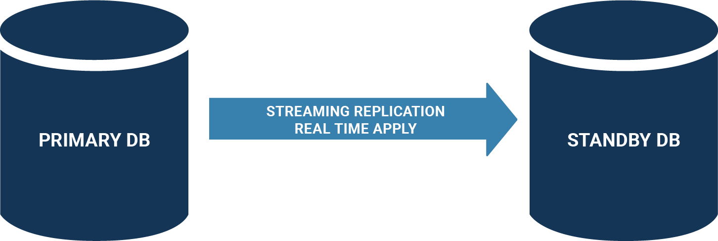
There are two types of replication available in PostgreSQL at the moment: Streaming replication & Logical replication. If you are looking to set up streaming replication for PostgreSQL 13, this is the page you have been looking for. This tutorial will show you how to configure PostgreSQL replication and how to set up your database servers quickly.
Before we get started with configuring PostgreSQL, it makes sense to take a look at what we want to achieve. The goal of this tutorial is to create a primary server replicating data to a secondary one, using asynchronous replication.
The entire setup will be done using CentOS 8.3. The process on RHEL (Redhat Enterprise Linux) is expected to be the same. Simply follow the same procedures.
Let’s prepare these systems step-by-step.
Once you have installed CentOS / RHEL you can already prepare the installation of PostgreSQL itself. The way to do that is to go to the PostgreSQL website and follow the instructions.
The following script shows how things work. You can simply copy / paste the script:
|
1 2 3 4 5 6 7 8 9 10 11 |
sudo dnf install -y https://download.postgresql.org/pub/repos/yum/reporpms/EL-8-x86_64/pgdg- redhat-repo-latest.noarch.rpm sudo dnf -qy module disable postgresql sudo dnf install -y postgresql13-server # can be skipped on the 2nd node sudo /usr/pgsql-13/bin/postgresql-13-setup initdb sudo systemctl enable postgresql-13 # can be skipped on the 2nd node sudo systemctl start postgresql-13 |
|
1 2 3 4 5 6 7 8 9 10 |
[root@node1 ~]# ps axf | grep post 5542 pts/1 S+ 0:00 _ grep --color=auto post 5215 ? Ss 0:00 /usr/pgsql-13/bin/postmaster -D /var/lib/pgsql/13/data/ 5217 ? Ss 0:00 _ postgres: logger 5219 ? Ss 0:00 _ postgres: checkpointer 5220 ? Ss 0:00 _ postgres: background writer 5221 ? Ss 0:00 _ postgres: walwriter 5222 ? Ss 0:00 _ postgres: autovacuum launcher 5223 ? Ss 0:00 _ postgres: stats collector 5224 ? Ss 0:00 _ postgres: logical replication launcher |
Now let’s move on to the next step: disabling the firewall on the primary.
|
1 2 3 4 |
[root@node1 ~]# systemctl disable firewalld Removed /etc/systemd/system/multi-user.target.wants/firewalld.service. Removed /etc/systemd/system/dbus-org.fedoraproject.FirewallD1.service. [root@node1 ~]# systemctl stop firewalld |
Why is that necessary? The replica will connect to the master on port 5432. If the firewall is still active, the replica will not be able to access port 5432. In our example, the firewall will be disabled completely to make it easier for the reader. In a more secure setup, you might want to do this in a more precise manner.
There are four things we have to do on the primary server:
postgresql.confpg_hba.confWe can perform these things step-by-step.
postgresql.conf.The file can be found in /var/lib/pgsql/13/data/postgresql.conf. However, if you have no clue where to find postgresql.conf you can ask PostgreSQL itself to point you to the configuration file. Here is how it works:
|
1 2 3 4 5 6 7 8 9 10 |
[root@node1 ~]# su - postgres [postgres@node1 ~]$ psql postgres psql (13.2) Type 'help' for help. postgres=# SHOW config_file; config_file ---------------------------------------- /var/lib/pgsql/13/data/postgresql.conf (1 row) |
postgresql.conf:listen_addresses = '*'
What does listen_addresses mean? By default, PostgreSQL only listens on localhost. Remote access is not allowed by default for security reasons. Therefore, we have to teach PostgreSQL to listen on remote requests as well. In other words: listen_addresses defines the bind addresses of our database service. Without it, remote access is not possible (even if you change pg_hba.conf later on).
Then we can create the user in the database:
|
1 2 |
postgres=# CREATE USER repuser REPLICATION; CREATE ROLE |
Of course, you can also set a password. What is important here is that the user has the REPLICATION flag set. The basic idea is to avoid using the superuser to stream the transaction log from the primary to the replica.
The next thing we can do is to change pg_hba.conf, which controls who is allowed to connect to PostgreSQL from which IP.
host replication repuser 10.0.3.201/32 trust
We want to allow the repuser coming from 10.0.3.201 to log in and stream the transaction log from the primary. Keep in mind that 10.0.3.200 is the primary in our setup and 10.0.3.201 is the replica.
Finally, we can restart the primary because we have changed listen_addresses in postgresql.conf.
If you only changed pg_hba.conf a reload is enough:
|
1 2 3 |
[postgres@node1 ~]$ exit logout [root@node1 ~]# systemctl restart postgresql-13 |
Your system is now ready, and we can focus our attention on the replica.
The next step is to create the replica. There are various things we need to do to make this work. The first thing is to make sure that the replica is stopped and that the data directory is empty. Let’s first make sure the service is stopped:
|
1 |
[root@node2 ~]# systemctl stop postgresql-13 |
Then, we need to make sure the data directory is empty:
|
1 2 3 4 5 6 |
[root@node2 ~]# cd /var/lib/pgsql/13/data/ [root@node2 data]# ls PG_VERSION global pg_dynshmem pg_logical pg_replslot pg_stat pg_tblspc pg_xact postmaster.opts base log pg_hba.conf pg_multixact pg_serial pg_stat_tmp pg_twophase postgresql.auto.conf current_logfiles pg_commit_ts pg_ident.conf pg_notify pg_snapshots pg_subtrans pg_wal postgresql.conf [root@node2 data]# rm -rf * |
Note that this step is not necessary if you have skipped the initdb step during installation.
However, it is necessary if you want to turn an existing server into a replica.
|
1 2 3 4 5 |
[root@node2 data]# su postgres bash-4.4$ pwd /var/lib/pgsql/13/data bash-4.4$ pg_basebackup -h 10.0.3.200 -U repuser --checkpoint=fast -D /var/lib/pgsql/13/data/ -R --slot=some_name -C |
pg_basebackup will connect to the primary and simply copy all the data files over. The connection has to be made as repuser. To ensure that the copy process starts instantly, it makes sense to tell PostgreSQL to quickly checkpoint. The -D flag defines the destination directory where we want to store the data on the replica. The -R flag automatically configures our replica for replication.
No more configuration is needed on the secondary server. Finally, we created a replication slot. What is the purpose of a replication slot in PostgreSQL? Basically, the primary server is able to recycle the WAL - if it is not needed anymore on the primary. But what if the replica has not consumed it yet? In that case, the replica will fail unless there is a replication slot ensuring that the primary can only recycle the WAL if the replica has fully consumed it. We at CYBERTEC recommend to use replication slots in most common cases.
pg_basebackup has done:|
1 2 3 4 5 6 7 8 9 10 11 12 13 14 15 16 17 18 19 20 21 22 23 24 25 26 27 28 29 |
bash-4.4$ ls -l total 196 -rw-------. 1 postgres postgres 3 Feb 12 09:12 PG_VERSION -rw-------. 1 postgres postgres 224 Feb 12 09:12 backup_label -rw-------. 1 postgres postgres 135413 Feb 12 09:12 backup_manifest drwx------. 5 postgres postgres 41 Feb 12 09:12 base -rw-------. 1 postgres postgres 30 Feb 12 09:12 current_logfiles drwx------. 2 postgres postgres 4096 Feb 12 09:12 global drwx------. 2 postgres postgres 32 Feb 12 09:12 log drwx------. 2 postgres postgres 6 Feb 12 09:12 pg_commit_ts drwx------. 2 postgres postgres 6 Feb 12 09:12 pg_dynshmem -rw-------. 1 postgres postgres 4598 Feb 12 09:12 pg_hba.conf -rw-------. 1 postgres postgres 1636 Feb 12 09:12 pg_ident.conf drwx------. 4 postgres postgres 68 Feb 12 09:12 pg_logical drwx------. 4 postgres postgres 36 Feb 12 09:12 pg_multixact drwx------. 2 postgres postgres 6 Feb 12 09:12 pg_notify drwx------. 2 postgres postgres 6 Feb 12 09:12 pg_replslot drwx------. 2 postgres postgres 6 Feb 12 09:12 pg_serial drwx------. 2 postgres postgres 6 Feb 12 09:12 pg_snapshots drwx------. 2 postgres postgres 6 Feb 12 09:12 pg_stat drwx------. 2 postgres postgres 6 Feb 12 09:12 pg_stat_tmp drwx------. 2 postgres postgres 6 Feb 12 09:12 pg_subtrans drwx------. 2 postgres postgres 6 Feb 12 09:12 pg_tblspc drwx------. 2 postgres postgres 6 Feb 12 09:12 pg_twophase drwx------. 3 postgres postgres 60 Feb 12 09:12 pg_wal drwx------. 2 postgres postgres 18 Feb 12 09:12 pg_xact -rw-------. 1 postgres postgres 335 Feb 12 09:12 postgresql.auto.conf -rw-------. 1 postgres postgres 28014 Feb 12 09:12 postgresql.conf -rw-------. 1 postgres postgres 0 Feb 12 09:12 standby.signal |
pg_basebackup has copied everything over. However, there is more. The standby.signal file has been created which tells the replica that it is indeed a replica.
Finally, the tooling has adjusted the postgresql.auto.conf file, which contains all the configuration needed to make the replica connect to its replica on the primary server (node1):
|
1 2 3 4 5 6 7 |
bash-4.4$ cat postgresql.auto.conf # Do not edit this file manually! # It will be overwritten by the ALTER SYSTEM command. primary_conninfo = 'user=repuser passfile=''/var/lib/pgsql/.pgpass'' channel_binding=prefer host=10.0.3.200 port=5432 sslmode=prefer sslcompression=0 ssl_min_protocol_version=TLSv1.2 gssencmode=prefer krbsrvname=postgres target_session_attrs=any' primary_slot_name = 'some_name' |
Voilà, we are done and we can proceed to start the replica.
We are ready to start the replica using systemctl:
|
1 2 3 4 5 6 7 8 9 10 11 12 |
bash-4.4$ exit exit [root@node2 data]# systemctl start postgresql-13 [root@node2 data]# ps axf | grep post 36394 pts/1 S+ 0:00 _ grep --color=auto post 36384 ? Ss 0:00 /usr/pgsql-13/bin/postmaster -D /var/lib/pgsql/13/data/ 36386 ? Ss 0:00 _ postgres: logger 36387 ? Ss 0:00 _ postgres: startup recovering 000000010000000000000007 36388 ? Ss 0:00 _ postgres: checkpointer 36389 ? Ss 0:00 _ postgres: background writer 36390 ? Ss 0:00 _ postgres: stats collector 36391 ? Ss 0:00 _ postgres: walreceiver streaming 0/7000148 |
It’s a good idea to check that the processes are indeed running. It’s especially important to check for the existence of the walreceiver process. walreceiver is in charge of fetching the WAL from the primary. In case it is not there, your setup has failed.
Also make sure that the service is enabled.
Once the setup has been completed, it makes sense to take a look at monitoring. In general, it makes sense to use a tool such as pgwatch2 to professionally monitor your database.
|
1 2 3 4 5 6 7 8 9 10 11 12 13 14 15 16 17 18 19 20 21 22 23 24 25 26 27 28 29 |
[root@node1 ~]# su - postgres [postgres@node1 ~]$ psql postgres psql (13.2) Type 'help' for help. postgres=# x Expanded display is on. postgres=# SELECT * FROM pg_stat_replication ; -[ RECORD 1 ]----+------------------------------ pid | 6102 usesysid | 16385 usename | repuser application_name | walreceiver client_addr | 10.0.3.201 client_hostname | client_port | 34002 backend_start | 2021-02-12 09:27:59.53724-05 backend_xmin | state | streaming sent_lsn | 0/7000148 write_lsn | 0/7000148 flush_lsn | 0/7000148 replay_lsn | 0/7000148 write_lag | flush_lag | replay_lag | sync_priority | 0 sync_state | async reply_time | 2021-02-12 09:29:49.783076-05 |
The existence of a row in pg_stat_replication tells us that WAL is flowing from the primary to a secondary.
|
1 2 3 4 5 6 7 8 9 10 11 12 13 14 15 16 17 18 19 20 21 22 23 24 25 26 27 28 29 30 31 32 33 34 35 36 |
[root@node2 data]# su - postgres [postgres@node2 ~]$ psql postgres psql (13.2) Type 'help' for help. postgres=# x Expanded display is on. postgres=# SELECT * FROM pg_stat_wal_receiver; -[ RECORD 1 ]---------+-------------------------------------------- pid | 36391 status | streaming receive_start_lsn | 0/7000000 receive_start_tli | 1 written_lsn | 0/7000148 flushed_lsn | 0/7000148 received_tli | 1 last_msg_send_time | 2021-02-12 09:29:59.683418-05 last_msg_receipt_time | 2021-02-12 09:29:59.674194-05 latest_end_lsn | 0/7000148 latest_end_time | 2021-02-12 09:27:59.556631-05 slot_name | some_name sender_host | 10.0.3.200 sender_port | 5432 conninfo | user=repuser passfile=/var/lib/pgsql/.pgpass channel_binding=prefer dbname=replication host=10.0.3.200 port=5432 fallback_application_name=walreceiver sslmode=prefer sslcompression=0 ssl_min_protocol_version=TLSv1.2 gssencmode=prefer krbsrvname=postgres target_session_attrs=any |
A row in pg_stat_wal_receiver ensures that the WAL receiver does indeed exist, and that data is flowing.
That’s it! I hope you have enjoyed this tutorial. For more information on choosing between synchronous and asynchronous replication, take a look at this page.
Analysing data within PostGIS is just one side of the coin. What about publishing our datasets as maps that various clients can consume and profit from with Geoserver and PostGIS? Let’s have a look at how this can be accomplished with Geoserver. Geoserver acts in this regard as a full-fledged open source mapping server, supporting several OGC compliant services, such as OGC Web Mapping (WMS) or Web Feature Service (WFS).
OGC is an abbreviation for Open GIS Consortium, which is a community working on improving access to spatial information by developing standards in this area.
Here’s a quick overview of this article’s structure:
Let’s first start by setting up Geoserver as a single, non-clustered instance. For our demo, I recommend using one of the available Docker images to start up quickly. The steps listed below show how to pull our geoserver image (kartoza) first, and subsequently start the container with its default configuration within a tmux session, which allows us to easily monitor geoserver’s output.
docker pull kartoza/geoserver:2.18.2
tmux
docker run -it --name geoserver -p 8080:8080 -p 8600:8080 kartoza/geoserver:2.18.2
If everything runs smoothly, Apache Tomcat reports back with
org.apache.catalina.startup.Catalina.start Server startup in XX ms
In one of my last blog posts, I imported a csv containing locations of airports (https://ourairports.com/data/airports.csv). Let’s build on this and use these point geometries as the main vector layer for our visualization.
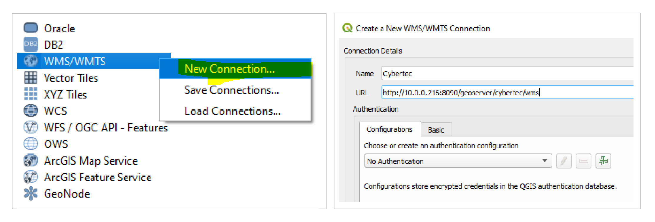
By using kartoza’s image defaults, Apache Tomcat will listen on port 8080 serving Geoserver’s web-interface with http://10.0.0.216:8090/geoserver. So, let’s continue and login with geoserver/admin.
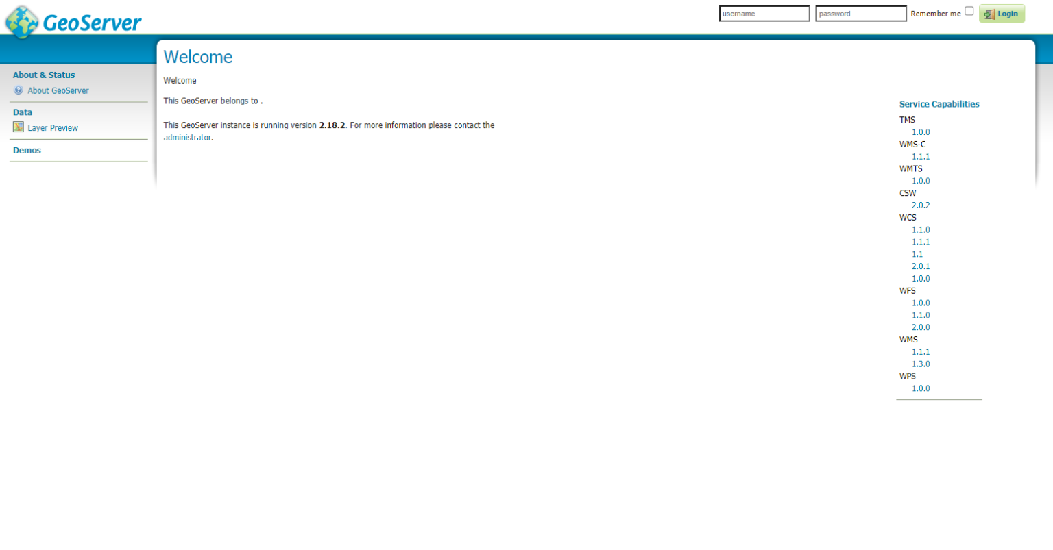
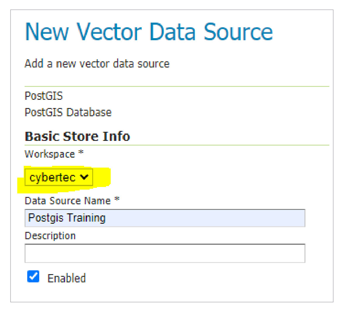
Figure 1 represents Geoserver’s main web screen after logging in. To publish our airport dataset, we must register our PostGIS database as a store (data source). To do so, I would first like to introduce the concept of workspaces within Geoserver. Workspaces are containers which data stores, layers and services belong to. Workspaces can be configured in detail in terms of accessibility and functionality.
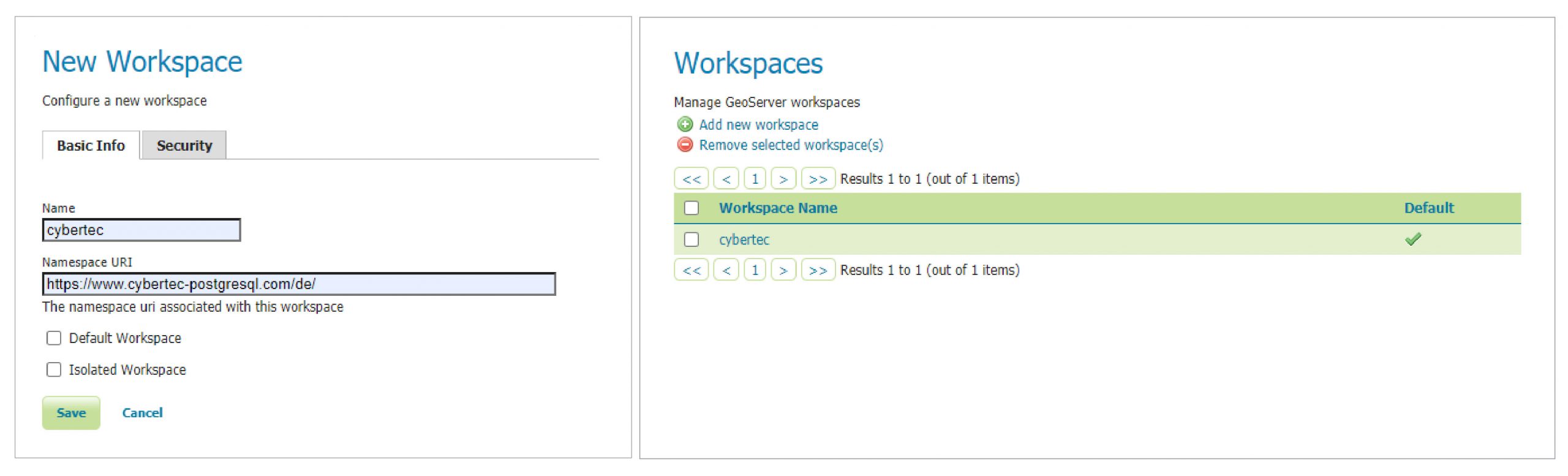
Setting up at least one workspace is required. Check out Figure 2 and 3 to understand how this can easily be accomplished.
Let’s come back to our initial task, and configure our PostGIS database as a vector data source.
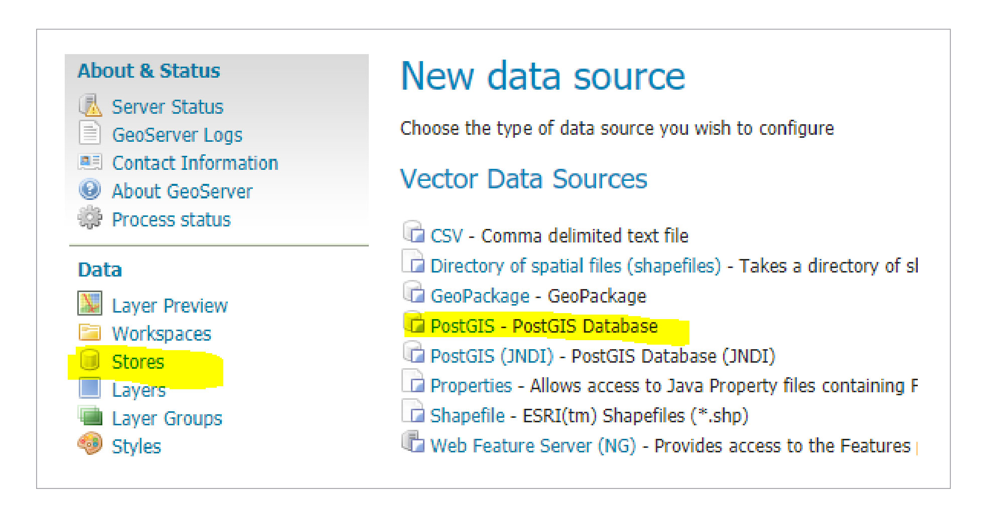
1. Click on store and choose PostGIS as your vector datasource:
2. Choose your workspace and configure and relate your PostGIS connection:
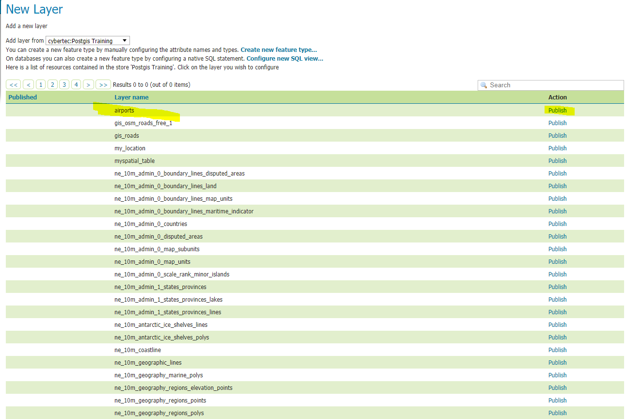
3. If everything runs according to plan, saving our new data source results in a list of available spatial tables. Picking airports from this list brings us one step closer to our goal.
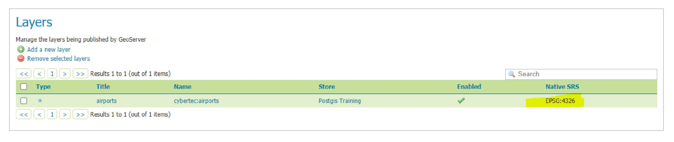
Unfortunately, we are not completely done with our initial layer configuration ☹. Successfully publishing a vector layer within Geoserver involves defining at least the coordinate reference system’s and layer’s extent (bounding box). Geoserver tries to extract the coordinate reference system from the data source’s metadata, thus if registered correctly within your data source, there should be no need to define this by hand. Subsequently, the layer’s bounding box can be extracted from the coordinate reference systems’ real data, or can be overridden too. Don’t worry about forgetting to define those parameters – Geoserver will force you to define these mandatory settings. Once the job has been done, you are rewarded for your efforts by finding a “fully” configured layer item in the layers section.
As mentioned in the beginning, Geoserver acts as a full-fledged open source mapping server. What do I mean by calling Geoserver full-fledged? On the one hand, I’m referring to its huge list of supported data sources and formats, on the other hand this statement is based on the wide range of spatial services implemented. By default, Geoserver is prebuilt with support for the following services: TMS, WMS-C, WMTS, CSW, WCS, WFS, WMS, and WPS. What do all these abbreviations mean? Most of them are acronyms for OGC-compliant services. But no worries – I won’t bother you with details of OGC standards – this time ????.Today and in this article, we will have a closer look at Web Mapping Services (WMS), but I recommend to check out OGC standards, released in https://www.ogc.org/docs/is, to get a comprehensive understanding what those services are about.
WMS stands for Web Mapping Service, which is an OGC-compliant mapping service whose main purpose is simply producing maps. WMS creates maps on the fly; this fact enables clients to individualize their map requests in terms of styling, extent and projection.
Within Geoserver, WMS is enabled globally by default, thus we can move on and test our service. Fortunately, Geoserver offers a useful layer preview, which allows us to verify various services within its own ecosystem.
Let’s open the Layer preview from the navigation pane and pick WMS/JPEG from the formats dropdown.
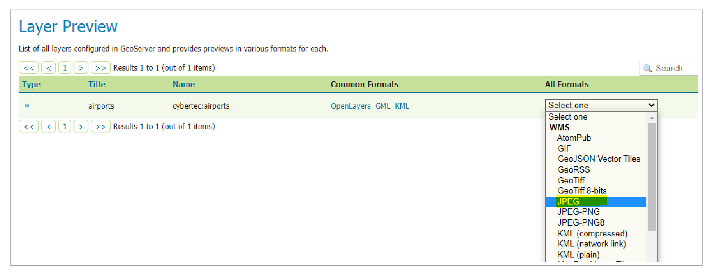
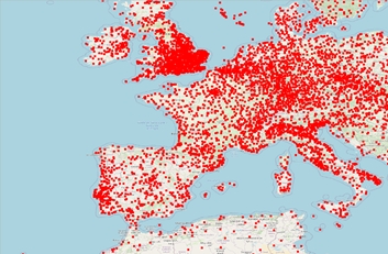
This action immediately results in a get request against our WMS endpoint, which responds with an image representing our airports.
http://10.0.0.216:8090/geoserver/cybertec/wms?service=WMS&version=1.1.0&request=GetMap&layers=cybertec%3Aairports&bbox=-179.8769989013672%2C-90.0%2C179.9757080078125%2C82.75&width=768&height=368&srs=EPSG%3A4326&styles=&format=image%2Fjpeg
Figure 9 presents the map generated. Not quite appealing you might think – I must agree. As we did not define and refine any styling parameters for our airport layer, Geoserver applies default stylings to our layer. Styling is another big story which will not be covered today.

It’s time to request our Web Mapping Service from our preferred GIS client. I am a huge fan of Quantum GIS (QGIS), a mature open-source GIS client, but any other fat or web-based client with WMS support will do this job too.
After opening up QGIS, add and configure a new WMS connection from the navigation pane (see Figure 10 and 11). By utilizing the layer preview, we can easily extract the http address our WMS listens to from the url which was previously generated.
http://10.0.0.216:8090/geoserver/cybertec/wms
What happens now in the background is quite interesting. QGIS first requests http://10.0.0.216:8090/geoserver/cybertec/wms?service=WMS&version=1.1.0&request=GetCapabilities, to gather comprehensive metadata about the service. The xml document it returns covers details about published layers, projections, formats and much more.
If everything has gone to plan, QGIS processes GetCapabilities response first and finally extends the WMS' description by our airport layer. Figure 12 proudly presents the results from our demonstration – airports which are displayed on top of OpenStreetMap tiles to slightly improve the overall map style.
We set up and configured Geoserver to publish an individual spatial dataset via WMS. By offering various data sources and OGC-compliant services out of the box, it’s no exaggeration to claim that Geoserver is a very powerful mapping server. This makes it easy to start and build up your spatial infrastructure. When it comes to productive environments, things turn out differently, since further topics such as performance and security must be considered too. If you would like more information on how to build up or improve your spatial infrastructure together with Geoserver and PostGIS, get in contact with the folks at CYBERTEC!
In PostgreSQL, every database connection is a server-side process. This makes PostgreSQL a robust multi-process rather than a multi-threaded solution. However, occasionally people want to terminate database connections. Maybe something has gone wrong, maybe some kind of query is taking too long, or maybe there is a maintenance window approaching.
In this blog you will learn how to terminate queries and database connections in PostgreSQL.
In PostgreSQL there are two functions we need to take into consideration when talking about cancellation or termination:
pg_cancel_backend(pid): Terminate a query but keep the connection alivepg_terminate_backend(pid): Terminate a query and kill the connectionpg_cancel_backend ist part of the standard PostgreSQL distribution and can be used quite easily:
|
1 2 3 4 5 6 7 8 9 10 11 12 13 14 15 16 17 18 |
test=# x Expanded display is on. test=# df+ pg_cancel_backend List of functions -[ RECORD 1 ]-------+--------------------------------------- Schema | pg_catalog Name | pg_cancel_backend Result data type | boolean Argument data types | integer Type | func Volatility | volatile Parallel | safe Owner | hs Security | invoker Access privileges | Language | internal Source code | pg_cancel_backend Description | cancel a server process' current query |
As you can see, all that’s necessary is to pass the process ID (pid) to the function. The main question is therefore: How can I find the ID of a process to make sure that the right query is cancelled?
The solution to the problem is a system view: pg_stat_activity.
|
1 2 3 4 5 6 7 8 9 10 11 12 13 14 15 16 17 18 19 20 21 22 23 24 25 |
test=# d pg_stat_activity View 'pg_catalog.pg_stat_activity' Column | Type | Collation | Nullable | Default ------------------+--------------------------+-----------+----------+--------- datid | oid | | | datname | name | | | pid | integer | | | leader_pid | integer | | | usesysid | oid | | | usename | name | | | application_name | text | | | client_addr | inet | | | client_hostname | text | | | client_port | integer | | | backend_start | timestamp with time zone | | | xact_start | timestamp with time zone | | | query_start | timestamp with time zone | | | state_change | timestamp with time zone | | | wait_event_type | text | | | wait_event | text | | | state | text | | | backend_xid | xid | | | backend_xmin | xid | | | query | text | | | backend_type | text | | | |
There are a couple of things to mention here: First of all, you might want to kill a query in a specific database. The “datname” field shows you which database a connection has been established to. The “query” column contains the query string. Usually this is the best way to identify the query you want to end. However, the fact that the “query” column contains a string does not mean that the affiliated command is actually active at the moment. We also need to take the “state” column into consideration. “active” means that this query is currently running. Other entries might indicate that the connection is waiting for more user input, or that nothing is happening at all.
“leader_pid” is also important: PostgreSQL supports parallel query execution. In case of a parallel query, parallelism is also executed using separate processes. To see which process belongs to which query, the “leader_pid” gives us a clue.
Once the query has been found, we can do the following:
|
1 2 3 4 5 6 7 8 9 10 11 12 |
test=# SELECT pg_cancel_backend(42000); pg_cancel_backend ------------------- t (1 row) test=# SELECT pg_cancel_backend(42353); WARNING: PID 42353 is not a PostgreSQL server process pg_cancel_backend ------------------- f (1 row) |
In case the query has been cancelled properly, we will get “true”. However, if the query is not there anymore, or in case the database connection does not exist, “false” will be returned.
So far, you have seen how a query can be ended. However, how can we terminate the entire connection?
Here is the definition of the function we will need for this purpose:
|
1 2 3 4 5 6 7 8 9 10 11 12 13 14 15 16 |
test=# df+ pg_terminate_backend List of functions -[ RECORD 1 ]-------+--------------------------- Schema | pg_catalog Name | pg_terminate_backend Result data type | boolean Argument data types | integer Type | func Volatility | volatile Parallel | safe Owner | hs Security | invoker Access privileges | Language | internal Source code | pg_terminate_backend Description | terminate a server process |
Calling it works according to the same concept as shown before. The following listing shows an example of how this can be done:
|
1 2 3 4 5 |
test=# SELECT pg_terminate_backend(87432); pg_terminate_backend ---------------------- t (1 row) |
However, sometimes kicking out a single user is not enough.
More often than not, we have to terminate all database connections except our own. Fortunately, this is reasonably easy to do. We can again use pg_stat_activity:
|
1 2 3 4 5 6 7 8 9 10 |
test=# SELECT pg_terminate_backend(pid) FROM pg_stat_activity WHERE pid <> pg_backend_pid() AND datname IS NOT NULL AND leader_pid IS NULL; pg_terminate_backend ---------------------- t t (2 rows) |
The first thing to exclude in the WHERE clause is our own PID which can be determined using the pg_backend_pid() function;
|
1 2 3 4 5 |
test=# SELECT pg_backend_pid(); pg_backend_pid ---------------- 75151 (1 row) |
The next important filter is to exclude database names which are NULL. Why is that important? In old versions of PostgreSQL, the system view only provided us with information about database connections. Current versions also list information about other processes. Those processes are not associated with a database (e.g. the background writer) and therefore we should exclude those. The same is true for parallel worker processes. Parallel workers will die anyway if we kill the parent process.
If you are interested in security, I would like to recommend “PostgreSQL TDE” which is a more secure version of PostgreSQL, capable of encrypting data on disk. It can be downloaded from our website. In addition to that, CYBERTEC offers 24x7 product support for PostgreSQL TDE.