Our PostgreSQL blog about “Speeding up count(*)” was widely read and discussed by our followers on the internet. We also saw some people commenting on the post and suggesting using different means to speed up count(*). I want to specifically focus on one of those comments and to warn our readers.

max(id) - min(id) will return the wrong answer

As stated in our previous post, count(*) has to read through the entire table to provide you with a correct count. This can be quite expensive if you want to read through a large table. So why not use an autoincrement field along with max and min to speed up the process? Regardless of the size of the table.

Here is an example:

This approach also comes with the ability to use indexes.

… can be indexed. PostgreSQL will look for the first and the last entry in the index and return both numbers really fast (if you have created an index of course - the serial column alone does NOT provide you with an index or a unique constraint).

Using sequences: What can possibly go wrong?

The question now is: What can possibly go wrong? Well … a lot actually. The core problem starts when transactions enter the picture. On might argue “We don't use transactions”. Well, that is wrong. There is no such thing as “no transaction” if you are running SQL statements. In PostgreSQL every query is part of a transaction - you cannot escape.

That leaves us with a problem:

So far so good …

Let us add a row and commit:

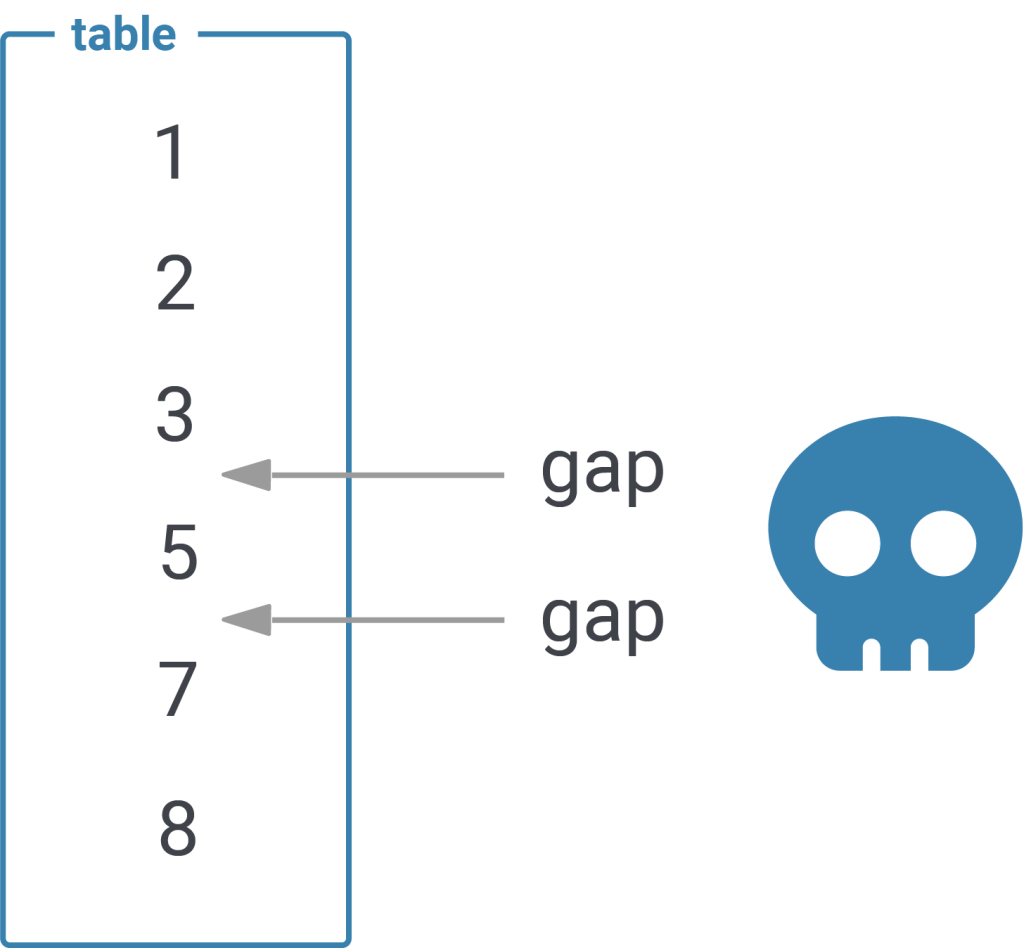
The important part is that a sequence DOES NOT assure that there are no gaps in the data - it simply ensures that the number provided will go up. Gaps are possible:

In my example “4” is missing which of course breaks our “count optimization”:

What you should learn from this example is that you should NEVER use sequences to speed up count(*). To make it clear: In PostgreSQL count(*) has to count all the data - there is no way around it. You might be able to estimate the content of the table, but you won't be able to calculate a precise row count with any of those tricks.

Finally...

If you want to take a look at Laurenz Albe's blog post, directly check it out on our website. If you want to learn more about performance in general check out our latest extension: pg_show_plans.

Last time I announced we would check out MobilityDB to improve our approach to extract overlapping passage times of healthy and infected individuals – here we go!

MobilityDB itself is a PostgreSQL extension built on top of PostGIS, specializing on processing and analysing spatio-temporal data. To do so, the extension adds a bunch of types and functions on top of PostGIS to solve different kinds of spatial-temporal questions.

Please check out Documentation (mobilitydb.com) to get an impression of what you can expect here.
The extension is currently available for PostgreSQL 11, PostGIS 2.5 as v1.0-beta version, whereby I understood from the announcements that we can definitely expect a first version to be released in early 2020. To quick start, I definitely recommend using their docker container codewit/mobility.

The blog-post is structured as follows:

1. Set up data structures within PostgreSQL (MobilityDB enabled)
2. Set up trips based on our initial mobile_points
3. Intersection of infected individual to retrieve possible contacts

Data structures of MobilityDB

As reminder, table mobile_points is a relic of our first blog-post and contains points of individuals. This table and its contents will be used to set up trajectories forming our trips. Table mobile_trips represent trips of individuals, whereas trips are modelled as trajectories utilizing MobilityDB’s tgeompoints data type. Instances of traj are generated from trip’s geometry and subsequently used for visualization.

Trip generation

Let’s start by generating trips out of points:

For each customer, a trip as sequence of instants of tgeompoint is generated. tgeompoint acts as continuous, temporal type introduced by MobilityDB. A sequence of tgeompoint interpolates spatio-temporally between our fulcrums. Here I would like to refer to MobilityDB’s documentation with emphasis on temporal types to dig deeper.

Figure 1 shows, not surprisingly, a visualization of resulting trip geometries (traj).

Analysis and results MobilityDB

Let’s start with our analysis and identify spatio-temporally overlapping segments of individuals. The following query returns overlapping segments (within 2 meters) by customer pairs represented as geometries.

To do so and to utilize spatio-temporal indexes on trips, expanded bounding-boxes are intersected first.

Next, we evaluate if trips overlap spatio-temporally by filtering:

getTime returns a detailed temporal profile of overlapping sections as set of periods constrained by tdwithin. A period is hereby a custom type introduced by MobilityDB, which is a customized version of tstzrange. Subsequently to extract intersecting spatial segments of our trip only, periodset restricts our trip by utilizing atPeriodSet. Finally, getValues extracts geometries out of tgeompoint returned by atPeriodSet.

But we’re not done. Multiple disjoint trip segments result in multi-geometries (Figure 2, 2 disjoint segments for customer 1 and 2). To extract passage times by disjoint segment and customer, multi-geometries must be “splitted up” first. This action can be carried out utilizing st_dump. To extract passage times for resulting simple, disjoint geometries, periods of periodset must be related accordingly.

This can be accomplished as follows:

First we turn our periodset into an array of periods. Next, we flatten the array utilizing unnest.
In the end, we call timespan on periods to gather passage times by disjoint segment.

Please find attached to the end of the article an even more elegant, improved way to extract passage times by disjoint trip segment utilizing MobilityDB’s functions only.

Visualization of results

The image below now shows results for both queries by highlighting segments of contact for our individuals in blue, labelled by its passage times.

So far so good – results correspond with our initial approach from my last blogpost.

What happens if we now remove some of our fulcrums and re-generate our trips?

Remember what I mentioned in the beginning regarding interpolation?

Figure 3 represents our generalized sequence of points, Figure 4 presents resulting trips, whose visualization already indicates that interpolation between points worked as expected. So even though we removed a bunch of fulcrums, resulting passage times correspond with our initial assessment (see figure 5).

Let’s go one step further...

and change the customers' speeds by the manipulation point’s timestamps in the beginning of one of ours trips only (figure 6 and 7). Figure 8 gives an impression, how this affects our results.

I just scratched the surface to showcase MobilityDB’s capabilities, but hopefully I made you curious enough to take a look by yourselves.
I (to be honest), already have felt in love with this extension and definitely will continue exploring.

Big respect for this great extension and special thanks goes to Esteban Zimanyi and Mahmoud Sakr, both main contributors, for their support!

Check out my other GIS posts:

• Let's Party and Upgrade PostgreSQL and PostGIS Together
• Intersecting Tracks of Individuals - MobilityDB
• Analyzing Historical Flight Data with MobilityDB

You may also be interested in free OpenStreetMap data:

• Open Street Map: Open GIS Data for your business

---

In order to receive regular updates on important changes in PostgreSQL, subscribe to our newsletter, or follow us on Facebook or LinkedIn.

By Kaarel Moppel - UPDATED by Laurenz Albe 06.07.2023 - See what progress has been made

What are PostgreSQL's weaknesses? How can PostgreSQL be improved? Usually, in this blog I write about various fun topics around PostgreSQL - like perhaps new cool features, some tricky configuration parameters, performance of particular features or on some “life hacks” to ease the life of DBA-s or developers. This post will be quite different though. It's inspired by an article called "10 Things I Hate about PostgreSQL" which I stumbled upon recently. I thought I’d also try my hand at writing about some less flattering sides of PostgreSQL 🙂 And yes, there are some, for sure - as with any major piece of software.

In the article I referenced, quite a few points are debatable from a technology viewpoint. However, in general I enjoyed the idea of exploring the dark side of the moon once in a while. Especially in our relational database domain, where problems tend to be quite complex - since there’s a bunch of legacy code out there (PostgreSQL has been around sind 1996!), there are the official SQL standards to be adhered to, and there are a gazillion different database / OS / hardware combinations out there in the wild.

So yeah, you definitely shouldn’t get blinded and praise any product X univocally. Especially given that the software world has gotten so complex and is moving so fast nowadays, that my guess is that nobody actually has the time to try out and learn all those competing technologies to a sufficiently good level. Well maybe only in academia, where one is not expected to directly start generating $$, the faster the better.

To love it or to hate it, that is the question

About the title - although it was kind of tempting to also use the word “hate” (more clicks probably), I found it too harsh in the end. In general - PostgreSQL is a truly well written and maintained software project, with a healthy Open Source community around it and it is also my default database recommendation for most applications. Its price - performance ratio is just yet to be beaten in the RDBMS sphere I believe. And there are far more benefits than shortcomings that I can think of.

The most important ones for me are its lightweightedness and simplicity for DBA operations (building a replication server is a one-liner!). From the development side, it is maybe the fact that Postgres is at the very top when it comes to implementing the ISO SQL standard, so that PostgreSQL can't really become a bottleneck for you. You could migrate to something else with a reasonable amount of work. In this area, a lot of commercial competitors have no real interest in such qualities - would you want to make migrating away from your product easy, if it’s generating you tens of thousands of dollars per instance per year?

So in short, as concluded in the post referenced, you can’t go wrong with PostgreSQL for most applications. But anyways, here are some of my points that I think could be improved to make PostgreSQL even better. Most of them are rather minor complaints you’ll find, or just looking at the clouds and wishing for more.

Construction Site #1 - Rigid query planning

This is related to the “no hints dogma” from the blog post referenced above (not to forget about the “pg_hint_plan” 3rd party extension though!) one of my biggest gripes with Postgres when it comes to complex queries - is the mostly static query planner. Mostly here means that except for some extra logic on choosing plans for prepared statements and PL/pgSQL stored procedures (which basically also boil down to prepared statements), the planner / execution doesn’t gather any feedback from the actual runs!

It pretty much cold-heartedly looks at the query, the pre-calculated statistics of tables mentioned in there, and then selects a plan and sticks to whatever happens. This holds true even if the row estimate for the first executed node is a million times off and some millions of rows are now going to be passed higher via a nested loop join, an algorithm that’s rather meant for handling small to medium datasets.

I do understand that employing some adaptive query planning strategies is a huge task. It would require decent resources to tackle it. However, some simple heuristics like automatic re-analyze based on seen data, or trying some other join types in the presented example should be probably doable as “low hanging fruits”. And it seems some people are already trying out such ideas already also - there’s for example the AQO project. But for real progress some wider cooperation would be probably needed to keep up with the big commercial products, who already throw around buzzwords like “AI-based query optimization”. Not sure if just marketing though or they really have something, not much stuff on that on the interwebs.

Could be improved: #2 Some levels of automatic tuning

Slightly connected to the first point is the idea of PostgreSQL automatically selecting some better values for default parameters, based on statistics gathered over time. Alternatively, it could just look at available OS resources. Currently, Postgres actually tries hard on purpose not to know too much about the OS (to support almost all platforms out there). For some reasonable subset of platforms and configuration settings, it could be done - theoretically.

I'm not talking about complex stuff even, but just the main things, like: optimizing the checkpoint settings (after some safety time + warnings), if checkpoints occur too often, increase autovacuum aggressiveness in case there’s lots of data changes coming in, look at memory availability and increase work_mem to get rid of some temp files, or enable wal_compression if the CPU is sitting idle. Currently, I think the only parameter that is automatically tuned / set is the “wal_buffers” parameter.

Well, in general, the topic of tuning is not a real problem for seasoned DBA's. Actually, the opposite is true - it’s our bread 🙂 However, it would surely benefit most developers out there. Also, this is what the competition is already touting. In the long run, this would benefit the project hugely, since DBA's are kind of a scarce resource nowadays, and extensive tuning could be off-putting for a lot of developers.

Still waiting on #3: Lost statistics during pg_upgrade

I’m sure most people have not heard or seen this issue, so it can’t really be described as a major problem. It has to do with the fact that old table statistics are not carried over when migrating to a newer Postgres version using the pg_upgrade utility, which is the fastest way to migrate, by the way. The original post talks about some hours of downtime... but with the “--link” flag, it’s usually less than a minute!

As I said, it’s not a biggie for most users that have ample downtime for upgrades or have only normal simple queries, selecting or updating a couple of rows over an index. On the other hand, for advanced 24/7 shops with lots of data, it can be quite annoying. It’s hard to predict the kind of spikes you’re going to get during those first critical minutes after an upgrade, when statistics are still being rebuilt. So here, it would be actually really nice if the statistics would not be “just deleted“ with every release, but only when some incompatibilities really exist.

For some versions, I even looked at the pertinent structures (pg_statistic group of tables) and couldn’t see any differences. I think it’s just a corner case and hasn’t gotten enough attention. There are also alternatives. If you really want to avoid such “iffy” moments, you could use logical replication (v10 and above) instead of the good old “in-place” upgrade method. Some details on such upgrades can be found in this post about logical replication.

This one has gotten better: #4 Autovacuum and XID Wraparound - UPDATED

Also “featured” in the original post - historically speaking, the XID Wraparound and the seemingly randomly operated autovacuum background process have definitely been the number one problem for those who are not so up to date on how Postgres MVCC row versioning works, and haven’t tuned accordingly. At default settings, after some years of operation, given that transaction counts are also increasing steadily, it’s indeed very possible to have some downtime to take care of the gathered “debt”.

Still, I’d say it’s not so tragic for most people as it is depicted, as it affects only very busy databases. And if you’re running with version v9.6 of PostgreSQL or higher, then there’s a good chance that you’ll never get any wraparound-related downtime, because the algorithms are now a lot smarter. It has improved even more as of v12, where autovacuum is much more aggressive by default. You can do quick vacuums by skipping index maintenance!

To defend Postgres a bit - you can enable early warning signals for such situations (log_autovacuum_min_duration) and there are many internal statistics available...you just need to use this information and take action - the tools are there. But there’s definitely room for more improvement. For example, one cool idea (from my colleague Ants) would be to allow explicit declaration of “tables of interest” for long running snapshots. Currently, many autovacuum / wraparound problems are caused by the fact that long-running transactions, sadly, block pretty much all autovacuum cleanup activity within the affected database, even if we’re selecting a table that is completely static. Such declarations could probably also help on the replica side with reducing recovery conflict errors, making Postgres more load-balancing friendly.

FYI

- in this area there are also some very promising developments happening with the zHeap project, that aims to provide an alternative to the MVCC row storage model, reducing bloat and thereby surprises from the background processes like the autovacuum.

Notes to #4 by Laurenz Albe:

There have been major improvements in #4, although the fundamental problem is still there:

• in v13, we have autovacuum triggered by INSERT, which can trigger VACUUM earlier and reduce the magnitude of anti-wraparound autovacuum for INSERT-only tables (see this article about autovacuum and insert-only tables)
• From v14 on, anti-wraparound autovacuum skips index cleanup and removing dead tuples if things get dangerous (See more about this on github)

The second is the more important improvement, but the first is cooler.

On its way but not there yet... #5 Disk footprint and bloat - UPDATED

This is another well-acknowledged problem-area for PostgreSQL - its “on disk” footprint is mostly a bit higher than that of its competitors. Normally this doesn’t show in real life, since most of your “working data set” should be cached anyway, but it can gradually slow things down. This is especially true if you run at default configs or fail to do any manual maintenance from time to time. But luckily, some things are already happening in this area, like the zHeap project and also a new hybrid store (row + column storage) called ZedStore is emerging that will compress the data size considerably. It will make Postgres more suitable for ultra large data warehouses - so let’s hope it makes it into Postgres v14.

One could throw in here also the full compression topic...but in my opinion it’s not really that important for OLTP databases at least, as enterprise SSD disks are fast as hell nowadays, and you have the option to dabble on the file system level. For those rare use cases where 10TB+ data warehouses with near real-time analytical query expectations are needed, I’d maybe not recommend Postgres as a default anyway. There are better specialized systems which employ hybrid and columnar storage approaches for such needs; automatic block compression alone would not save us there.

Not to say that automatic compression is a bad idea, though: for example, the latest versions of TimescaleDB (a 3rd party PostgreSQL extension for time-series data) employ such tricks, can reduce the “on disk” size dramatically, and thereby speed up heavier queries. There’s also another extension called cstore_fdw. It's an extension for data warehouse use cases, so there are already options out there for Postgres.

Notes by Laurenz:

For #5, v13 has somewhat improved things with index de-duplication (at least B-tree indexes with duplicates take less space now).
That is only a slight step in the right direction, however.

#6 Out-of-the-box vulnerability against brute force password attacks - UPDATED

I put this one in even though there’s been some thought put into it, since there’s a “contrib” (bundled with Postgres) extension named “auth_delay” for exactly this purpose. What's true about Postgres out of the box - there’s no limit on password login attempts! Also, by default, users can open up to $max_connections (minus some superuser reserved connections) sessions in parallel...this could mean trouble if you have some mean gremlins in your network. Note, however, that under “password login” I mean “md5” and “scram-256” auth methods, meaning if you forward your authentication to LDAP or AD, you should be safe - but be sure to validate that. Or, you could enable the “auth_delay” extension; better safe than sorry! It’s really easy to crack weak passwords if you know the username -  basically a one-liner! So it would be really nice to see some kind of soft limits kick in automatically.

N.B.! This doesn’t mean that you don’t get notified of the failed login attempts, but it could be too late if you don't monitor the log files actively! P.S.: there’s also an extension which deals with the same “problem space”, called pg_auth_mon and we (CYBERTEC) also have a patch for support customers to disable such attacked accounts automatically after X failed attempts.

Don't forget though - by default, access config Postgres only listens to connections from the localhost, so the potential threat only occurs if some IP range is made explicitly accessible!

Notes by Laurenz:

For #6,

• v14 has changed password_encryption to scram-sha-256 by default, which makes brute force attacks way harder, since scram hashes are more expensive.
• v16 has introduced (or will introduce) require_auth, which allows the client to reject unsafe authentication methods and makes identity theft by faking the server way harder..

Finally, #7: No query cache

This is one of those “wishing for more” or “nice to have” items on my list. The general idea behind it is that it’s quite wasteful to execute exactly the same deterministic query (fixed parameters, immutable functions etc) and scan some large tables fully every time, returning exactly the same results - if the data hasn't changed! There are probably some non-obvious technical pitfalls lurking around here...but some databases have managed to implement something like that. MySQL now decided to retire it in v8.0 due to some unfortunate implementation details...so the stuff is not easy.  However, since performance is the main thing that developers (especially junior ones) worry about, and given that Postgres materialized views are also not always useful, something like that would be an awesome addition.

That should do

Phew...that was tiring already. Seems it’s not really that easy to find 10 things to improve about PostgreSQL...because it’s a really solid database engine 🙂 So let’s stop at 7 this time, but if you have some additional suggestions, please leave a comment. Hope it broadened your (database) horizons, and do remember to decide on the grand total of pluses and minuses.

Read more about PostgreSQL performance and data types in Laurenz Albe's blog: UNION ALL, Data Types and Performance

 

Most people know that autovacuum is necessary to get rid of dead tuples. These dead tuples are a side effect of PostgreSQL's MVCC implementation. So many people will be confused when they read that from PostgreSQL v13 on, commit b07642dbc adds support for autovacuuming insert-only tables (also known as “append-only tables”).

This article explains the reasons behind that and gives some advice on how to best use the new feature. It will also explain how to achieve similar benefits in older PostgreSQL releases.

Note that all that I say here about insert-only tables also applies to insert-mostly tables, which are tables that receive only few updates and deletes.

How insert-triggered autovacuum works

From v13 on, PostgreSQL will gather statistics on how many rows were inserted since a table last received a VACUUM. You can see this new value in the new “n_ins_since_vacuum” column of the pg_stat_all_tables catalog view (and in pg_stat_user_tables and pg_stat_sys_tables).

Autovacuum runs on a table whenever that count exceeds a certain value. This value is calculated from the two new parameters “autovacuum_vacuum_insert_threshold” (default 1000) and “autovacuum_vacuum_insert_scale_factor” (default 0.2) as follows:

where reltuples is the estimate for the number of rows in the table, taken from the pg_class catalog.

Like other autovacuum parameters, you can override autovacuum_vacuum_insert_threshold and autovacuum_vacuum_insert_scale_factor with storage parameters of the same name for individual tables. You can disable the new feature by setting autovacuum_vacuum_insert_threshold to -1.

You can use “toast.autovacuum_vacuum_insert_threshold” and “toast.autovacuum_vacuum_insert_scale_factor” to change the parameters for the associated TOAST table.

Use case 1: “anti-wraparound” vacuum on insert-only tables

Why do insert-only tables need VACUUM?

PostgreSQL stores transaction IDs in the xmin and xmax system columns to determine which row version is visible to which query. These transaction IDs are unsigned 4-byte integer values, so after slightly more than 4 billion transactions the counter hits the upper limit. Then it “wraps around” and starts again at 3.

As described in this blog post, that method would cause data loss after about 2 billion transactions. So old table rows must be “frozen” (marked as unconditionally visible) before that happens. This is one of the many jobs of the autovacuum daemon.

Why anti-wraparound vacuum on insert-only tables can be a problem

The problem is that PostgreSQL only triggers such “anti-wraparound” runs once the oldest unfrozen table row is more than 200 million transactions old. For an insert-only table, this is normally the first time ever that autovacuum runs on a table. There are two potential problems with that:

• The anti-wraparound vacuum doesn't get done in time. Then, one million transactions before it would suffer data corruption, PostgreSQL will not accept any new transactions. You have to start it in single-user mode and run VACUUM manually. You can find a description of such cases in this and this blog.
• Different from other autovacuum runs, anti-wraparound autovacuum will not give up when it blocks a concurrent transaction. This will block even short operations that require an ACCESS EXCLUSIVE lock (like DDL statements on the table). Such a blocked operation will block all other access to the table, and processing comes to a standstill. You can find such a case described in this blog.

How to protect yourself from disruptive anti-wraparound vacuums

From PostgreSQL v13 on, the default settings should already protect you from this problem. This was indeed the motivation behind the new feature.

For PostgreSQL versions older than v13, you can achieve a similar effect by triggering anti-wraparound vacuum earlier, so that it becomes less disruptive. For example, if you want to vacuum a table every 100000 transactions, you can set this storage parameter:

If all tables in your database are insert_only, you can reduce the overhead from autovacuum by setting vacuum_freeze_min_age to 0, so that tuples get frozen right when the table is first vacuumed.

Use case 2: index-only scans on insert-only tables

How index-only scans work in PostgreSQL

As mentioned above, each row contains the information for which transactions it is visible. However, the index does not contain this information. Now if you consider an SQL query like this:

where you have an index on id, all the information you need is available in the index. So you should not need to fetch the actual table row (“heap fetch”), which is the expensive part of an index scan. But unfortunately you have to visit the table row anyway, just to check if the index entry is visible or not.

To work around that, PostgreSQL has a shortcut that makes index-only scans possible: the visibility map. This data structure stores two bits per 8kB table block, one of which indicates if all rows in the block are visible to all transactions. If a query scans an index entry and finds that the block containing the referenced table row is all-visible, it can skip checking visibility for that entry.

So you can have index-only scans in PostgreSQL if most blocks of a table are marked all-visible in the visibility map.

The problem with index-only scans on insert-only tables

Since VACUUM removes dead tuples, which is required to make a table block all-visible, it is also VACUUM that updates the visibility map. So to have most blocks all-visible in order to get an index-only scan, VACUUM needs to run on the table often enough.

Now if a table receives enough UPDATEs or DELETEs, you can set autovacuum_vacuum_scale_factor to a low value like 0.005. Then autovacuum will keep the visibility map in good shape.

But with an insert-only table, it is not as simple to get index-only scans before PostgreSQL v13. One report of a problem related to that is here.

How to get index-only scans on insert-only tables

From PostgreSQL v13 on, all you have to do is to lower autovacuum_vacuum_insert_scale_factor on the table:

In older PostgreSQL versions, this is more difficult. You have two options:

• schedule regular VACUUM runs with cron or a different scheduler
• set autovacuum_freeze_max_age low for that table, so that autovacuum processes it often enough

Use case 3: hint bits on insert-only tables

In PostgreSQL, the first query that reads a newly created row has to consult the commit log to figure out if the transaction that created the row was committed or not. It then sets a hint bit on the row that persists that information. That way, the first reader saves future readers the effort of checking the commit log.

As a consequence, the first reader of a new row “dirties” (modifies in memory) the block that contains it. If a lot of rows were recently inserted in a table, that can cause a performance hit for the first reader. Therefore, it is considered good practice in PostgreSQL to VACUUM a table after you insert (or COPY) a lot of rows into it.

But people don't always follow that recommendation. Also, if you want to write software that supports several database systems, it is annoying to have to add special cases for individual systems. With the new feature, PostgreSQL automatically vacuums insert-only tables after large inserts, so you have one less thing to worry about.

Future work

During the discussion for the new feature we saw that there is still a lot of room for improvement. Autovacuum is already quite complicated (just look at the many configuration parameters) and still does not do everything right. For example, truly insert-only tables would benefit from freezing rows right away. On the other hand, for tables that receive some updates or deletes as well as for table partitions that don't live long enough to reach wraparound age, such aggressive freezing can lead to unnecessary I/O activity.

One promising idea Andres Freund propagated was to freeze all tuples in a block whenever the block becomes dirty, that is, has to be written anyway.

The fundamental problem is that autovacuum serves so many different purposes. Basically, it is the silver bullet that should solve all of the problems of PostgreSQL's MVCC architecture. That is why it is so complicated. However, it would take a major redesign to improve that situation.

Conclusion

While it seems to be an oxymoron at first glance, autovacuum for insert-only tables mitigates several problems that large databases used to suffer from.

In a world where people collect “big data”, it becomes even more important to keep such databases running smoothly. With careful tuning, that was possible even before PostgreSQL v13. But autovacuum is not simple to tune, and many people lack the required knowledge. So it is good to have new autovacuum functionality that takes care of more potential problems automatically.

 

(Updated 2023-02-22) In my daily work, I see many databases with a bad setting for max_connections. There is little advice out there for setting this parameter correctly, even though it is vital for the health of a database. So I decided to write up something.

What is max_connections?

According to the documentation, max_connections determines the maximum number of concurrent connections to the database server. But don't forget that superuser_reserved_connections of these connections are for superusers only (so that superusers can connect even if all other connection slots are blocked). With the default setting of 100 and 3 for these parameters, there are 97 connections open for application purposes.

Since PostgreSQL reserves shared memory for all possible connections at server start, you have to restart PostgreSQL after changing max_connections.

Why do people choose high values for max_connections?

There are several reasons:

• Since you need a restart to increase max_connections, people want to be “on the safe side”.
• People got the error
  ERROR: remaining connection slots are reserved for non-replication superuser connections
  and raised the limit so that they don't get the error anymore.
• The application developers convinced the DBA that they need many database connections for best performance.

It seems like an easy enough solution to increase the number of connections.

What are the problems of high values for max_connections?

Setting max_connections to a high value can have severe consequences:

Risk of overloading the database

As long as all but three of your 500 database sessions are idle, not much harm is done. Perhaps taking the snapshot at the beginning of each query is a little slower, but you probably won't notice that.

But there is nothing that can prevent 100 of the connections from becoming active at the same time. Perhaps a particular event occurred (everybody wants to buy a ticket the minute after sales started). Perhaps a rogue statement kept a lock too long and processes ready to run “piled up” behind the lock.

If that happens, your CPU and/or I/O subsystem will be overloaded. The CPU will be busy switching between the processes or waiting for I/O from the storage subsystem, and none of your database sessions will make much progress. The whole system can “melt down” and become unresponsive, so that all you can do is reboot.

Obviously, you don't want to get into that situation, and it is not going to improve application performance either.

Insufficient resources for each database connection

There is a limited amount of RAM in your machine. If you allow more connections, you can allot less RAM to each connection. Otherwise, you run the danger of running out of memory. The private memory available for each operation during query execution is limited by work_mem. So you will have to set this parameter low if you use a high value for max_connections.

Now work_mem has a direct influence on query performance: sorting will be faster if it can use enough RAM, or PostgreSQL may prefer a faster hash join or hash aggregate and avoid a sort at all.

So setting max_connections high will make queries perform slower than they could, unless you want to risk running out of memory.

Is high max_connections always bad?

If you read the previous section carefully, you will see that it is not actually max_connections that is the problem. Rather, you want a limit on the actual number of connections. max_connections is just an upper limit for that number. While it is important not to have too many client connections, it is also a bad idea to enforce that limit with max_connections, because exceeding that limit will cause application errors.

We will see below that a connection pool is the best way to enforce a limit on the number of active sessions. Then there is no danger of too many connections, and there is no need to set max_connections particularly low. On the contrary: if your application is set up for high availability and fails over to a different application server, it can take a while for the old client connections to time out on the server. Then it can be important to set max_connections high enough to accommodate the double number of client connections for a while.

An upper limit for the number of database connections

You want to utilize your resources without overloading the machine. So your setting should satisfy

• num_cores is the number of cores available
• parallel_io_limit is the number of concurrent I/O requests your storage subsystem can handle
• session_busy_ratio is the fraction of time that the connection is active executing a statement in the database
• avg_parallelism is the average number of backend processes working on a single query.

The first two numbers are easy to obtain, and you usually have a good idea if you will use a lot of parallel query or not. But session_busy_ratio can be tricky to estimate. If your workload consists of big analytical queries, session_busy_ratio can be up to 1, and avg_parallelism will be one more than max_parallel_workers_per_gather. If your workload consists of many short statements, session_busy_ratio can be close to 0, and avg_parallelism is 1.

Often you will have to use a load test to determine the best value of max_connections by experiment. The aim is to keep the database busy, but not overloaded.

For some workloads, this formula or an experiment would lead to a high setting for max_connections. But you still shouldn't do that, as stated above: the more connections you have, the bigger the danger of many connections suddenly becoming active and overloading the machine. The better solution in this case is to use a connection pool to increase session_busy_ratio.

Using a connection pool

A connection pool is a piece of software that keeps a number of persistent database connections open. It uses these connections to handle database requests from the front-end. There are two kinds of connection pools:

• Connection pools built into the application or the application server. Rather than opening a database connection, application processes request a connection from the pool. When they are done, they return it to the pool rather than closing the connection.
• External connection pools like pgBouncer. Such a connection pool looks like a database server to the front end. SQL statements from the application are executed over a limited number of backend connections to the database.

Connection pools provide an artificial bottleneck by limiting the number of active database sessions. Using them increases the session_busy_ratio. This way, you can get by with a much lower setting for max_connections without unduly limiting your application.

Conclusion

It is important for the health and performance of your application not to have too many open database connections.

If you need to be able to handle many database connections due to architecture limitations (the application server has no connection pool, or there are too many application servers), use a connection pooler like pgBouncer. Then you can give each connection the resources it needs for good performance.

If you want to know how to best size your connection pool, you could read my article on that topic.

In times of COVID-19, governments contemplate tough measures to identify and trace infected people. These measures include the utilization of mobile phone data to trace down infected individuals and subsequently contacts to curb the epidemic. This article shows how PostGIS’ functions can be used to identify “overlapping” sections of infected and healthy individuals by analysing tracks spatio-temporally.
This time we don’t focus on performance and tuning, rather strive boosting your creativity on PostgreSQL’s spatial extension and its functionalities.

The article is structured as follows:

1. Set up data structures within PostgreSQL
2. Set up sample tracks via QGIS
3. Segment sample tracks to retrieve induvial track points
4. Intersection of infected individual to retrieve possible contacts

Data structures of GPS tracks

Let’s start by defining tables representing tracks and their points.
Table mobile_tracks acts as a helper table storing artificial tracks of individuals, which have been drawn via QGIS.
Table mobile_points stores points, which result from segmenting tracks. Finally, they have been enriched by timestamps, which are used to identify temporal intersections on top of spatial intersections. 

The test area is located in Vienna/Austria; therefore I chose MGI/Austria 34 (EPSG as 31286) as appropriate projection.

GPS tracks and points

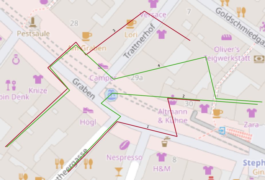
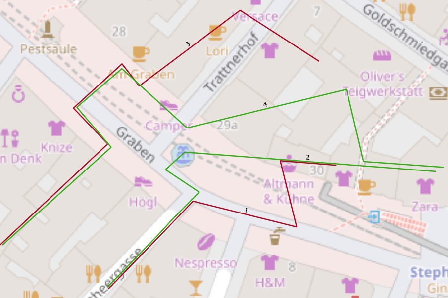
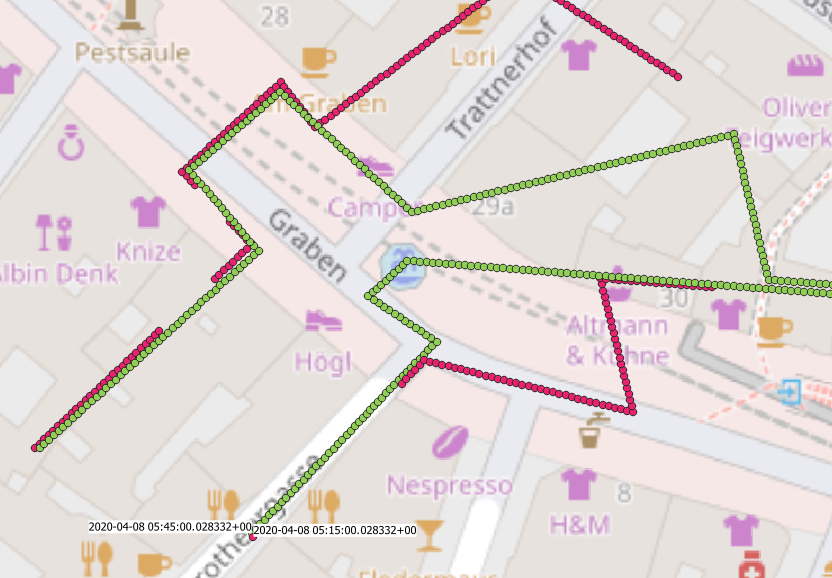
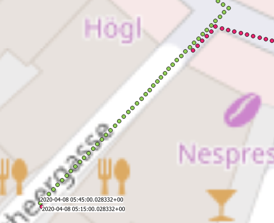
As mentioned in the beginning, for points I decided to generate artificial ones from tracks, I previously digitized via QGIS. Figure 1 shows tracks of infected people in red, healthy individuals are represented as green line strings as foundation.

For our simple example, I made the following assumptions:

• Individuals are moving with the same speed
• Tracks of individuals start at the same time

To extract individual points for tracks, I utilized PostGIS’s ST_Segmentize function as follows:

The query creates points every meter, timestamps are subsequently increased by 1000 milliseconds.

Identification of intersection points

Now it’s time to start with our analysis. Did our infected individual meet somebody?
Let’s start with an easy approach and select points of healthy individuals, which have been within 2 meters to infected individuals while respecting a time interval of 2 seconds. 

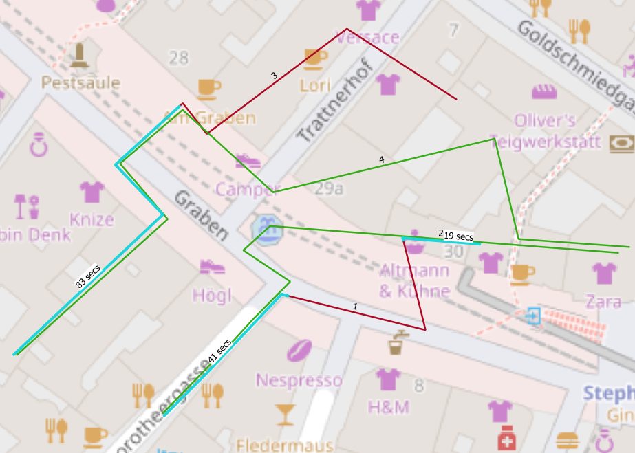
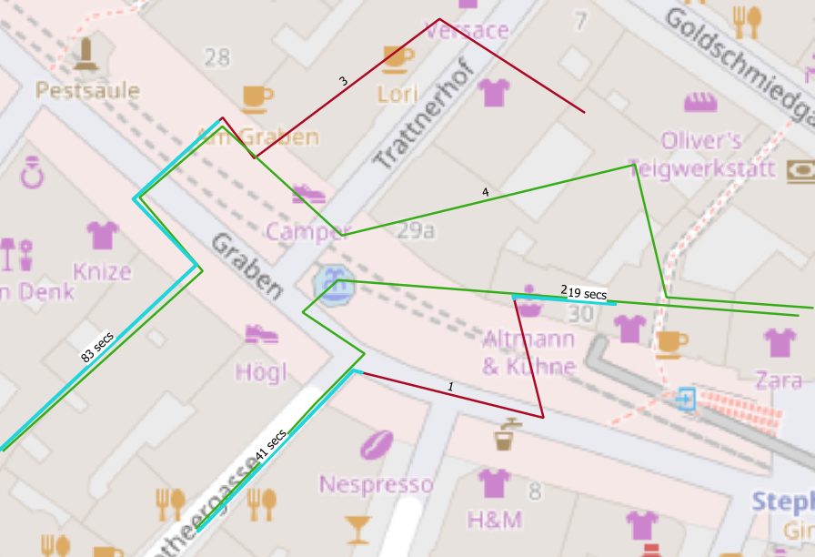
Figure 3 and 4 show results for the given query by highlighting points of contact for our individuals in blue. As mentioned before, this query covers the most basic solution to identify people who met.
Alternatively, PostGIS’ ST_CPAWithin and ST_ClosestPointOfApproach functions could be used here as well to solve this in a similar manner. To do so, our points must get modelled as trajectories first.

To refine our solution, let’s identify temporal coherent segments of spatial proximity and respective passage times. The goal is to understand, how long people have been close enough together to inherit possible infections more realistically. The full query is attached to the end of the post. 

Step 1 - aggregStep1

Based on our first query results, for each point we calculate the time interval to its predecessor. Considering our initial assumptions, a non-coherent temporal segment will lead to gaps >1 second.

Step 2 – aggregStep2

With our new column indicating the temporal gap between current and previous point, we cluster segments 

Step 3 – aggregStep3

For each cluster, we subtract min from max timestamp to extract a passage interval.

Step 4

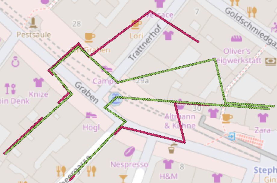
Finally, for each combination of infected/healthy individual, the segment with the maximum passage time is being extracted and a linestring is generated by utilizing st_makeline (see figure 7).

Even though results can serve as foundation for further analysis, our approach still remains constrained by our initially taken assumptions. 

Recently, a very promising PostgreSQL extension named MobilityDB has been published, which offers a lot of functionalities to solve all kinds of spatio-temporal related questions. Take a look at this blogpost to learn more.

By Kaarel Moppel

2 weeks ago we announced a new, long awaited, Postgres extension to look into execution plans for “live” running queries: pg_show_plans. This was not possible before in PostgreSQL yet, so it’s really a very cool piece of functionality and we’d like to echo out the message again. So here in this blogpost we’ll reiterate some basics but also explain some more implementation details. Let's take a detailed look on the new PostgreSQL troubleshooting extension:

The general idea

Although in general PostgreSQL is an absolutely solid database product from all angles (2 recent “RDBSM of the year” titles testify to that) - time to time on busy / volume heavy system there are hiccups - queries suddenly last longer than you think. Of course you could see some crucial details (who, how long, is someone blocking, the exact query) already easily via the built-in pg_stat_activity view or the historical behaviour fur such statements via pg_stat_statements...but what was missing so far, was the ability to look at the exact query plan chosen for that currently running slow query! Only after the query finished it was possible to analyze the root cause of slowness by re-executing manually with EXPLAIN or with the auto_explain extension, slightly inconveniently via logfiles. But lo and behold - now it’s possible to look at execution plans of slow queries via SQL also in real-time as they’re being executed!

Implementation idea

So what does this new pg_show_plans extension do exactly? In PostgreSQL terms - it copies query execution plan info from the private session / backend context to shared memory context when the query starts, so that it would be accessible also to other users. Using shared memory though requires “being there” when the server starts - so one needs to add the extension to the shared_preload_libraries list, optionally also configure some settings (see the configuration chapter below for details) and restart the server.

Installation

Currently the extension is provided to the public only as source code, so one needs to build it from sources. We of course provide RPM / DEB packages to all customers also in case needed. But building from sources is also very standard and painless if you're following the simple steps from the README or check out the previous blog post again where it’s compiled from any directory location. The README suggests going into the Postgres source folder.
Note that  Postgres versions 9.1 and upwards, till 13 beta are supported.

Configuration

As mentioned in the introductory chapter pg_show_plans needs to be there when the server starts to claim some shared memory and set up some executor event hooks so at least one line needs changing in the postgresql.conf or alternatively one ALTER SYSTEM command.

Besides that there are only a couple of parameters that could be of interest for more advanced users:

pg_show_plans.plan_format - controls the output format. By default it’s optimized for “humans looking at stuff”™ but if you plan to integrate with some visual query analyzing tool like PEV etc, you could opt for the JSON output. Luckily this can be altered on individual session level so robots and humans can even live peacefully side to side this time.

pg_show_plans.max_plan_length - to be by default light on the server resources EXPLAIN plan texts of up to 8kB (defined in bytes!) are only stored by default! So if having complex queries and seeing “” instead of plans, one could again opt to increase that value (1..100kB range) but bear in mind that this memory is reserved upfront for each connection slot (max_connections).

Now one can restart the PostgreSQL server and our extension is ready for usage.

Usage

Ok, so how to use this tool after we’ve installed and configured it? Well for those who have an abundance of well or “too well” loaded systems they can just take the last query below but for test purposes first I’ll first set up some test data to get a slowish query to kind of simulate real life conditions.

And the output that should help us understand the reasons for slow runtime:

pid	20556
level	0
userid	10
dbid	13438
plan	Aggregate  (cost=17930054460.85..17930054460.86 rows=1 width=8)   ->  Nested Loop  (cost=0.85..15430054460.85 rows=1000000000000 width=0)         ->  Index Only Scan using pgbench_accounts_pkey on pgbench_accounts a  (cost=0.42..25980.42 rows=1000000 width=0)         ->  Materialize  (cost=0.42..33910.43 rows=1000000 width=0)               ->  Index Only Scan using pgbench_accounts_pkey on pgbench_accounts b  (cost=0.42..25980.42 rows=1000000 width=0)

Ouch, a typo in the join condition...who wrote that? Better terminate that query….

In practice to make the output even more usable one might want to add also some minimum runtime filtering and instead of userid / dbid show real names - looking something like that:

Performance

As all extra activities inside the database have some kind of cost attached to them, a valid question would be - how “costly” it is to enable this extension and let it monitor the query “traffic”? Well, as so often in tech - it depends. On the busyness of your server i.e. how many concurrent queries are running and how long are they on average. For very parallel and short statements (<0.1ms) there’s indeed a penalty that one can notice ~ 20% according to my measurements with “pgbench” using the “--select-only” to get the micro-transactions. But for normal, more slowish real life queries the performance hit was small enough to be ignored. But in short - if having mostly very short queries, de-activate the extension by default (pg_show_plans_disable function) and then enable only when starting some kind of debugging sessions via the pg_show_plans_enable function.

Credits

The code was implemented by one of our PostgreSQL core hackers Suzuki Hironobu, who in turn was inspired by the existing pg_store_plans extension, so some credit is surely due to those fellas. Thanks a lot for making PostgreSQL better! Although it’s not something you’ll need every day, it’s something that advanced users look for and might select or ditch certain products because of that. Oracle for example has also had something similar available (v$sql_plan, v$sql_plan_monitor views) for some time, so a very welcome addition indeed.

Summary

As you saw - pg_show_plans is a very nice addition to PostgreSQL’s troubleshooting toolkit and simple enough to be used both by DBA-s and developers. It supports all remotely recent PostgreSQL versions and the best part - it’s Open Source under the PostgreSQL licence! Take it and use it however you see fit...but as always, we would of course be thankful for any kind of feedback, to improve this extension further.

GitHub project page here.

Also maybe good to know - our PostgreSQL monitoring tool of choice, pgwatch2, also has built-in support for this extension in real-time mode so you can easily display live EXPLAIN plan info for long-running queries nicely on a Grafana dashboards! A sample here:

By Kevin Speyer - Time Series Forecast - This post shows you how to approach a time series problem using machine learning techniques. Predicting the behavior of a variable over time is a common problem that one encounters in many industries, from prices of assets on the stock market to the amount of transactions per minute on a server. Despite its importance, time series forecasting is a topic often overlooked in Machine Learning. Moreover, many online courses don't mention the topic at all.

Time series analysis is particularly hard because there is a difficulty that doesn't occur with other problems in Machine Learning: The data has a particular order and it is highly correlated. This means that if you take two observations with the exact same attribute values, the outcome may be totally different due to the recent past measurements.

Implications

This has other practical implications when you attack the problem. For example, you can't split the data between training and validation sets like you would with typical machine learning problems, because the order of the data itself contains a lot of information. One correct way to split the data set in this case would be to keep the first 3/4 of the observations to train the model, and the final 1/4 to validate and test the model's accuracy. There are other more sophisticated ways to split the data, like the rolling window method, that we encourage the reader to look into.

In this case, we'll use the famous ARIMA model to predict the monthly industrial production of electric and gas utilities in the United States from the years 1985–2018. The data can be extracted from the Federal Reserve  or from kaggle.

The ARIMA model

The AutoRegressive Integrated Moving Average (ARIMA) is the go-to model for time series forecasting. In this case we assume that the behavior of the variable can be estimated only from the values that it has taken in the past and there are no external attributes that influence it (other than noise). These cases are known as univariate time series forecasting.

The ARIMA model is actually a combination of three algorithms:

AR: The AutoRegressive models are just linear regression models that fit the present value based on p previous values. The parameter p gives the number of back-steps that will be taken into account to predict the present value.

MA: The Moving Average model proposes that the output is a linear combination of the current and various past values of a random variable. This model assumes that the data is stationary in time, that is, that the average and the variance do not vary on time. The parameter in this case is the number of past values taken into account q

I: "Integrated" refers to the variable that will be fitted. Instead of trying to forecast the value of the observed variable, it is easier to forecast how different the new value will be with respect to the last one. This means using the difference between consecutive steps as the target variable instead of the observable variable itself. In lots of cases, this is an important step, because it will transform the current non-stationary time series into a stationary series. You can go one step further and use the difference of the difference as your target value. If this reminds you of calculus, you are on the right path! The parameter in this case (i) is the number of differentiating to be performed. i=1 means using the discrete derivative as the target variable, i=2 is using the discrete second derivative as the target variable, and so forth.

Exploring the data set

Loading the data:

Typically, we store data in databases, so the first thing we should do is establish a connection and retrieve it. It's easy to do in Python, use the libraries psycopg2 and pandas as follows:

The data consists of 397 records with no missing values. We will now split the data into 200 training values, 70 validation values and 127 test values. It is important to always maintain the order of the data, otherwise it will be impossible to perform a coherent forecast.

It's convenient to observe the training and validation data to observe the behavior of the energy production over time:

The first thing we can notice from this plot is that the data seems to have different components. On the one hand, the average mean value increases over time. On the other hand, there seems to be a high frequency modulation of energy production.

Fitting the data and forecast

Finally, it's time to adjust the model. We have three hyper-parameters (p, i and d) that we have to choose in order to get the best model possible. A good way to do this is simply to propose some values for the hyperparameters, adjust the model with the training data, and see how well each model performs when predicting the validation data. We call it hyperparameter optimization: don't, as is so often the case, do it wrong:

In hyperparameter optimization, the score of each model with different parameters should be obtained against the validation set, not against the training set.

In Python, this can be done in a couple of lines:

The output shows how well the model was able to predict the validation data for each set of parameters:

Here we can observe that the error is minimized by the parameters p=8, i=1 and q=12. Let's see how the forecast looks when compared to the actual data:

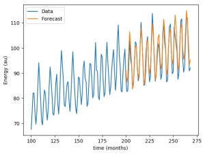
The newly adjusted model predicts the future values of energy prediction pretty well, it looks like we've succeeded!

The problem of predicting the future

Or did we? Now that we have an optimal set of hyperparameters, we should try our model with the test set. Now we take the training and the validation set to adjust our model with p=8, i=1 and q=12, and forecast the values of the test set that it has never seen.

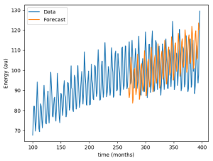
As it turns out, the forecast doesn't fit the data as well as we expected. The mean error went from 0.4 against validation data to 1.1 against test data, almost three times worse! The change in behavior in the data explains this. Energy production ceases to grow, which is something impossible to predict when looking only at the past data. Even for many fully deterministic problems, making predictions far into the future is an impossible task due to highly sensitive initial conditions.

See another of Kevin Speyer's machine learning posts: Series Forecasting with Recurrent Neural Networks (LSTM)

What are the performance differences between normal and generic audit triggers? Recently I was talking in a more general way about some common auditing / change tracking approaches for PostgreSQL...but it also made me curious, how does it look from the performance side?

To quickly recap the previous blog post: the most common approaches for tracking important changes are mostly solved with writing some triggers. There are two main variations: table specific triggers / audit tables and a more generic approach with only one trigger function and one (or also many) generic audit tables, usually relying on PostgreSQL’s NoSQL features that allow quite a high degree of genericness in quite a convenient and usable way.

Obviously one could “guesstimate” that the generic approach would perform worse than the tailored approach as this is commonly the case in software. But the question is - how much worse? Can it be considered negligible? Well there's only one way to find out I guess….and finally after finding some time to set up a small test case I can say that I was in for a bit of a surprise! But do read on for details or see the last paragraph for the executive summary.

Test schema for the “table specific” approach

I used pgbench to create auditing tables for the three pgbench tables that receive updates (detailed SQL here). It quickly generated SQL for the background auditing tables and attached triggers. While the schema is simple, I’m only including an excerpt here; the full script is available. I kept the history table populated by pgbench since it has no indexes and shouldn’t impact performance, ensuring both test cases remain equal.

Test schema for the “generic” approach

As with the explicit schema, we’re starting with the default pgbench schema but now extending it only with a single trigger function that will be attached to all 3 tables getting updates! And there will also only be a single logging table relying on the “generic” JSONB data type to handle all kinds of various inputs with just one column. Full SQL code below (or here):

Setup info

Some hardware / software information for completeness:

Test host: 4 CPU i5-6600, 16GB RAM, SATA SSD

PostgreSQL: v12.1, all defaults except shared_buffers set to 25% of RAM, i.e. 2GB, checkpoint_completion_target = 0.9, backend_flush_after = '2MB' (see here for explanation).

Pgbench: scale 1000, i.e. ~ 13GB DB size to largely factor out disk access (working set should fit more or less into RAM for good performance on any DB system), 4h runtime, 2 concurrent sessions (--jobs) not to cause any excessive locking on the smaller tables. Query latencies were measured directly in the database using the pg_stat_statement extension, so they should be accurate.

Results - TPS & latencies

Performance has many aspects but let’s start with TPS (Transactions per Second) and transaction latencies (single transaction duration) as they are probably the most important metrics for the performance hungry. Surprisingly it turned out that the generic NoSQL approach was quite a bit faster in total numbers! Whew, I didn’t expect that for sure. Note the “in total numbers” though...as updates on the 2 small tables were still a tiny bit slower still, but the costliest update a.k.a. the “heart” of the transaction (on pgbench_accounts table) was still significantly faster still. See below table for details.

	Explicit triggers	Generic triggers	Difference (%)
TPS	585	794	+35.7
Total transaction	6324546	8581130	+35.7
Mean time of UPDATE pgbench_accounts (ms)	1.1127	0.8282	-25.6
Mean time of UPDATE pgbench_branches (ms)	0.0493	0.0499	+1.3
Mean time of UPDATE pgbench_tellers (ms)	0.0479	0.0483	+1.0

Results - disk footprint

Well here the decision is very clear when looking at the resulting auditing table sizes after the tests finished - the grand total of tables representing the traditional / explicit approach are much smaller than the one big generic table! So this is definitely also worth considering if you’re building the next Amazon or such. We shouldn’t only look at absolute numbers here as we had 35% more transactions with the generic approach...so we should also factor that in. 

	Explicit triggers	Generic triggers	Difference (%)	TPS adjusted difference (%)
Total size of auditing tables (in MB)	1578	4255	+170	+109

Note that the table sizes don’t include indexes.

Quering

While not directly related to this test, an important aspect of planning change tracking is the need to efficiently access the audit trail. After experimenting with various schemas, the explicit audit table approach clearly outperforms others. It eliminates the need for JSONB syntax, which can be challenging for beginners, and offers better query performance for complex queries as data accumulates. Additionally, the generic approach consumes about twice the space, making it less suitable for frequent historical queries.

Also you will most probably need more targeted functional indexes on the JSONB column as I wouldn’t recommend to just index everything with a single GiN index - although it would be the simplest way to go, it only makes sense if you really perform searches on the majority of all “columns”.

Anyways it’s hard to say something definitive here as real life requirements will differ vastly I imagine, and the amount of indexes / data will be decisive.

Summary

My personal learning from this test - it's not over until the fat lady sings 🙂 My initial hunch on the performance cost of generic JSONB storing triggers was not correct this time and the performance is actually great! So one shouldn’t be afraid of this approach due to the performance hit...but if at all, rather due to disk “costs”...or due to possible woes when needing to actually query the gathered data in some complex ways.

By the way - if you’re wondering why the generic approach was actually faster, my best bet is that it has to do with (at least) 3 factors:

1) PostgreSQL JSONB implementation is very-very efficient

2) less PL/pgSQL parsing / planning as same trigger code is used three times

3) better CPU level data caching as we have less active / hot data blocks.

And as always - remember that when choosing between different approaches for your own project I always recommend testing with your exact schema / hardware as schemas vary vastly and a lot depends on data types used. This test was just one of the simpler examples.

Bonus idea - generic “differential” change auditing

After finishing my test I started wondering if it would be somehow possible to reduce the disk “cost” downside of this otherwise neat “generic” approach...and it actually wasn’t too hard to put together some trigger code that looks at the row data and logs only columns and values that are changed!

The core idea can be seen in the code below (full sample here) and also the first short testing looked quite promising actually - about 40% of disk space savings compared to the above described generic approach! So this could be definitely an interesting way to go. Thanks for reading!

Read more about PostgreSQL, triggers and performance, see this blog: Why Are My PostgreSQL Updates Getting Slower? By Laurenz Albe.